Lecture 6 Program Flow Analysis Forrest Brewer Ryan

Lecture 6 Program Flow Analysis Forrest Brewer Ryan Kastner Jose Amaral

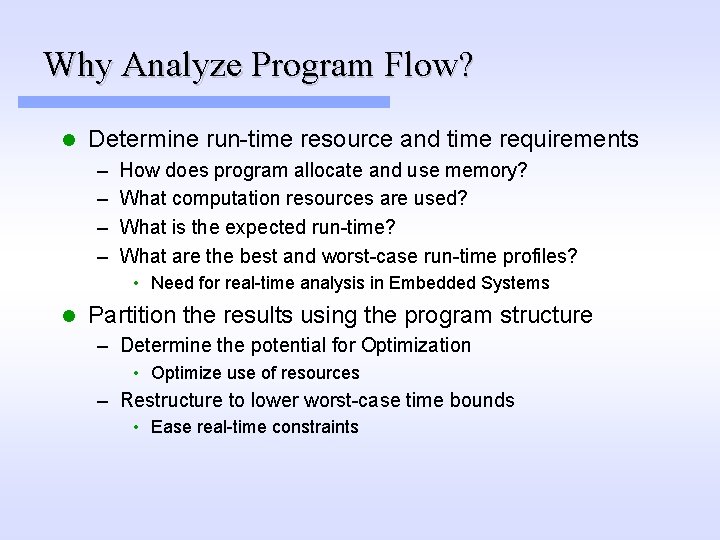
Why Analyze Program Flow? l Determine run-time resource and time requirements – – How does program allocate and use memory? What computation resources are used? What is the expected run-time? What are the best and worst-case run-time profiles? • Need for real-time analysis in Embedded Systems l Partition the results using the program structure – Determine the potential for Optimization • Optimize use of resources – Restructure to lower worst-case time bounds • Ease real-time constraints

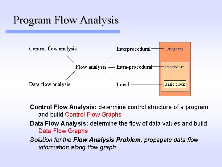
Program Flow Analysis Control flow analysis Flow analysis Data flow analysis Interprocedural Program Intra-procedural Procedure Local Basic block Control Flow Analysis: determine control structure of a program and build Control Flow Graphs Data Flow Analysis: determine the flow of data values and build Data Flow Graphs Solution for the Flow Analysis Problem: propagate data flow information along flow graph.

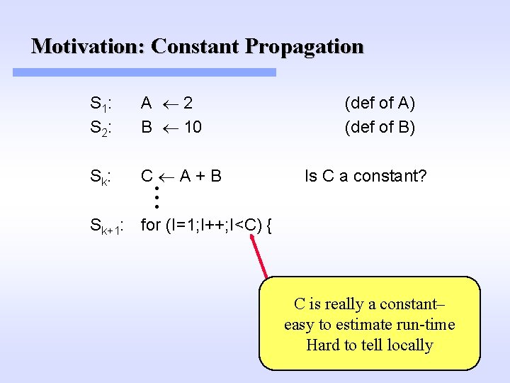
Motivation: Constant Propagation S 1: S 2: A 2 B 10 S k: C. A + B . . (def of A) (def of B) Is C a constant? Sk+1: for (I=1; I++; I<C) { C is really a constant– easy to estimate run-time Hard to tell locally

Code Optimizations Code optimization - a program transformation that preserves correctness and improves the performance (e. g. , execution time, size, resource contention, other metrics) of the input program. Code optimization may be performed at multiple levels of program representation: 1. Source code 2. Intermediate code 3. Target machine code Optimized vs. optimal - the term “optimized” is used to indicate a relative performance improvement. “Optimal” is a claim of non-inferiority among target set of programs.

Basic Blocks Def: A basic block is a sequence of consecutive intermediate language statements in which flow of control can only enter at the beginning and leave at the end. Only the last statement of a basic block can be a branch statement and only the first statement of a basic block can be a target of a branch. (Semantically, control branches and start targets take place only at beginning and end of basic blocks) (Aho. Sethi. Ullman, pp. 529)

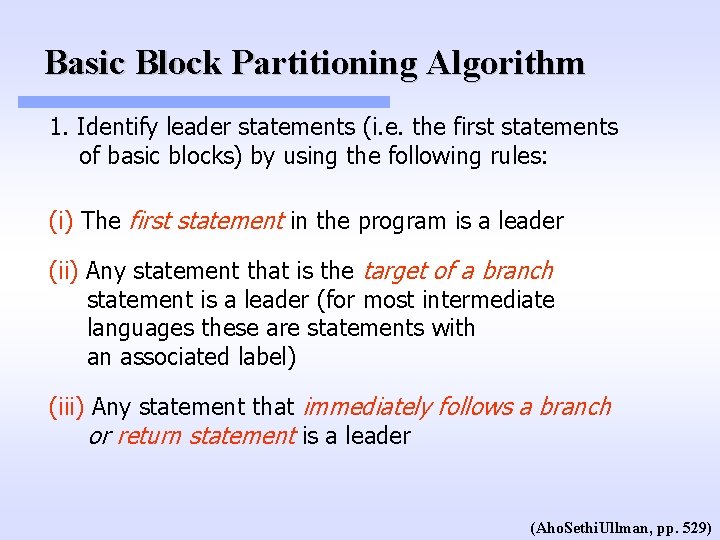
Basic Block Partitioning Algorithm 1. Identify leader statements (i. e. the first statements of basic blocks) by using the following rules: (i) The first statement in the program is a leader (ii) Any statement that is the target of a branch statement is a leader (for most intermediate languages these are statements with an associated label) (iii) Any statement that immediately follows a branch or return statement is a leader (Aho. Sethi. Ullman, pp. 529)

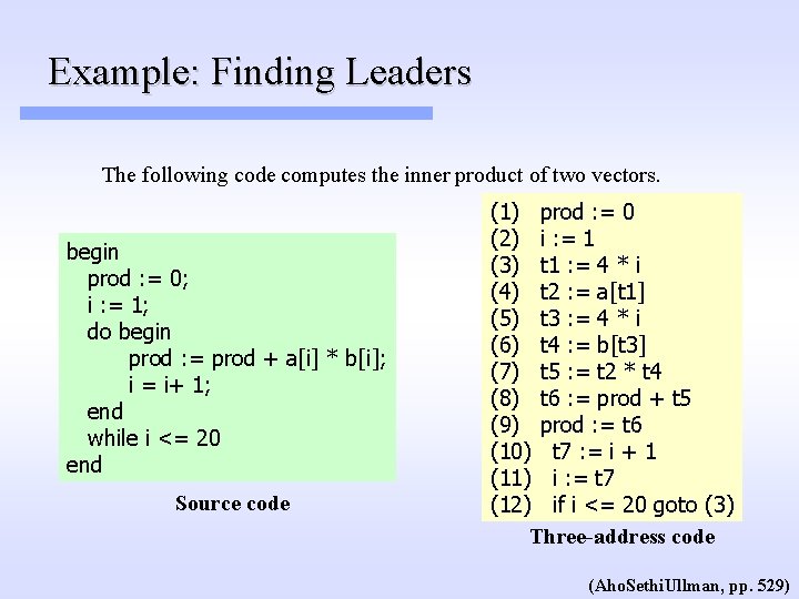
Example: Finding Leaders The following code computes the inner product of two vectors. begin prod : = 0; i : = 1; do begin prod : = prod + a[i] * b[i]; i = i+ 1; end while i <= 20 end Source code (1) prod : = 0 (2) i : = 1 (3) t 1 : = 4 * i (4) t 2 : = a[t 1] (5) t 3 : = 4 * i (6) t 4 : = b[t 3] (7) t 5 : = t 2 * t 4 (8) t 6 : = prod + t 5 (9) prod : = t 6 (10) t 7 : = i + 1 (11) i : = t 7 (12) if i <= 20 goto (3) Three-address code (Aho. Sethi. Ullman, pp. 529)

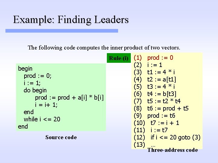
Example: Finding Leaders The following code computes the inner product of two vectors. Rule (i) (1) (2) begin (3) prod : = 0; (4) i : = 1; (5) do begin (6) prod : = prod + a[i] * b[i] (7) i = i+ 1; (8) end (9) while i <= 20 (10) end (11) Source code (12) (13) prod : = 0 i : = 1 t 1 : = 4 * i t 2 : = a[t 1] t 3 : = 4 * i t 4 : = b[t 3] t 5 : = t 2 * t 4 t 6 : = prod + t 5 prod : = t 6 t 7 : = i + 1 i : = t 7 if i <= 20 goto (3) … Three-address code

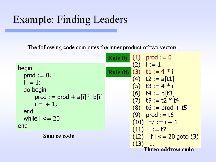
Example: Finding Leaders The following code computes the inner product of two vectors. Rule (i) (1) prod : = 0 (2) i : = 1 begin Rule (ii) (3) t 1 : = 4 * i prod : = 0; (4) t 2 : = a[t 1] i : = 1; (5) t 3 : = 4 * i do begin (6) t 4 : = b[t 3] prod : = prod + a[i] * b[i] (7) t 5 : = t 2 * t 4 i = i+ 1; (8) t 6 : = prod + t 5 end (9) prod : = t 6 while i <= 20 (10) t 7 : = i + 1 end (11) i : = t 7 Source code (12) if i <= 20 goto (3) (13) … Three-address code

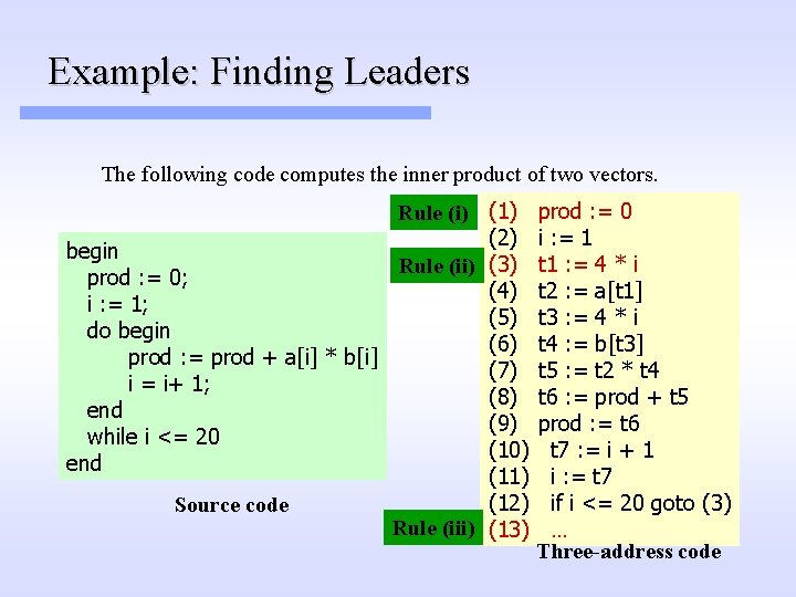
Example: Finding Leaders The following code computes the inner product of two vectors. Rule (i) (1) (2) begin Rule (ii) (3) prod : = 0; (4) i : = 1; (5) do begin (6) prod : = prod + a[i] * b[i] (7) i = i+ 1; (8) end (9) while i <= 20 (10) end (11) (12) Source code Rule (iii) (13) prod : = 0 i : = 1 t 1 : = 4 * i t 2 : = a[t 1] t 3 : = 4 * i t 4 : = b[t 3] t 5 : = t 2 * t 4 t 6 : = prod + t 5 prod : = t 6 t 7 : = i + 1 i : = t 7 if i <= 20 goto (3) … Three-address code

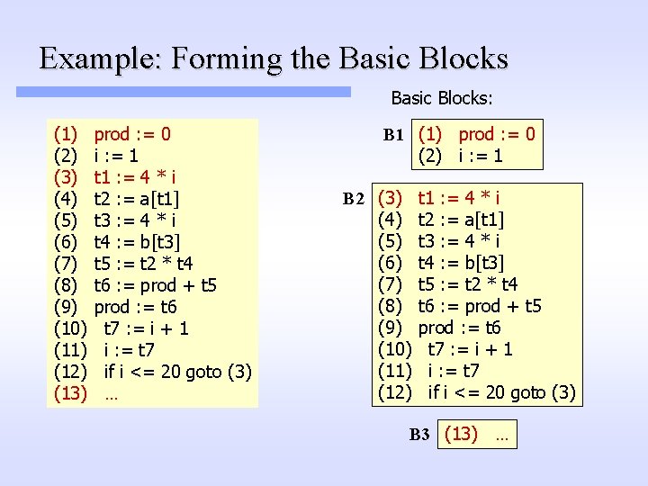
Example: Forming the Basic Blocks: (1) (2) (3) (4) (5) (6) (7) (8) (9) (10) (11) (12) (13) prod : = 0 i : = 1 t 1 : = 4 * i t 2 : = a[t 1] t 3 : = 4 * i t 4 : = b[t 3] t 5 : = t 2 * t 4 t 6 : = prod + t 5 prod : = t 6 t 7 : = i + 1 i : = t 7 if i <= 20 goto (3) … B 1 (1) prod : = 0 (2) i : = 1 B 2 (3) (4) (5) (6) (7) (8) (9) (10) (11) (12) t 1 : = 4 * i t 2 : = a[t 1] t 3 : = 4 * i t 4 : = b[t 3] t 5 : = t 2 * t 4 t 6 : = prod + t 5 prod : = t 6 t 7 : = i + 1 i : = t 7 if i <= 20 goto (3) B 3 (13) …

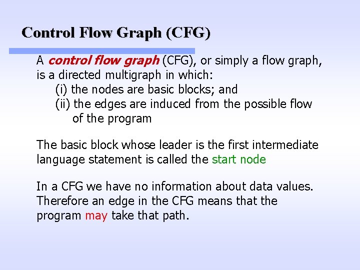
Control Flow Graph (CFG) A control flow graph (CFG), or simply a flow graph, is a directed multigraph in which: (i) the nodes are basic blocks; and (ii) the edges are induced from the possible flow of the program The basic block whose leader is the first intermediate language statement is called the start node In a CFG we have no information about data values. Therefore an edge in the CFG means that the program may take that path.

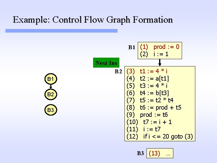
Example: Control Flow Graph Formation B 1 (1) prod : = 0 (2) i : = 1 B 2 B 3 Next Ins B 2 (3) (4) (5) (6) (7) (8) (9) (10) (11) (12) t 1 : = 4 * i t 2 : = a[t 1] t 3 : = 4 * i t 4 : = b[t 3] t 5 : = t 2 * t 4 t 6 : = prod + t 5 prod : = t 6 t 7 : = i + 1 i : = t 7 if i <= 20 goto (3) B 3 (13) …

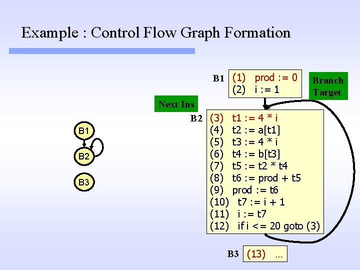
Example : Control Flow Graph Formation B 1 (1) prod : = 0 (2) i : = 1 B 2 B 3 Next Ins B 2 (3) (4) (5) (6) (7) (8) (9) (10) (11) (12) Branch Target t 1 : = 4 * i t 2 : = a[t 1] t 3 : = 4 * i t 4 : = b[t 3] t 5 : = t 2 * t 4 t 6 : = prod + t 5 prod : = t 6 t 7 : = i + 1 i : = t 7 if i <= 20 goto (3) B 3 (13) …

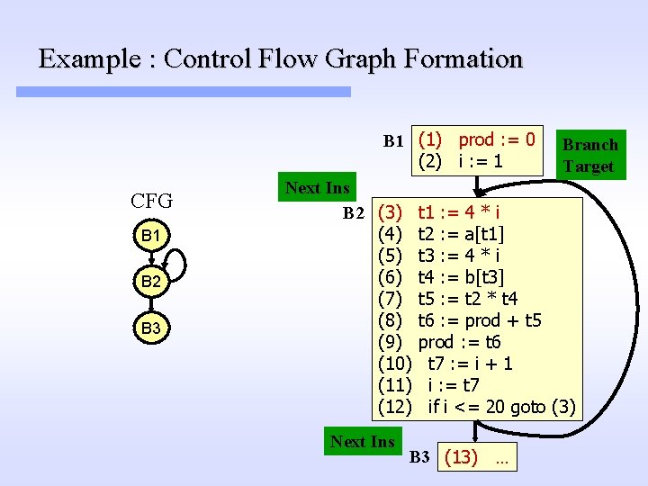
Example : Control Flow Graph Formation B 1 (1) prod : = 0 (2) i : = 1 CFG B 1 B 2 B 3 Next Ins B 2 (3) (4) (5) (6) (7) (8) (9) (10) (11) (12) Next Ins Branch Target t 1 : = 4 * i t 2 : = a[t 1] t 3 : = 4 * i t 4 : = b[t 3] t 5 : = t 2 * t 4 t 6 : = prod + t 5 prod : = t 6 t 7 : = i + 1 i : = t 7 if i <= 20 goto (3) B 3 (13) …

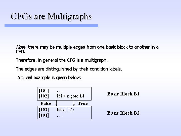
CFGs are Multigraphs Note: there may be multiple edges from one basic block to another in a CFG. Therefore, in general the CFG is a multigraph. The edges are distinguished by their condition labels. A trivial example is given below: [101] [102] False [103] [104] . . . if i > n goto L 1 Basic Block B 1 True label L 1: . . . Basic Block B 2

Identifying loops Question: Given the control flow graph of a procedure, how can we quickly identify loops? Answer: We use the concept of dominance.

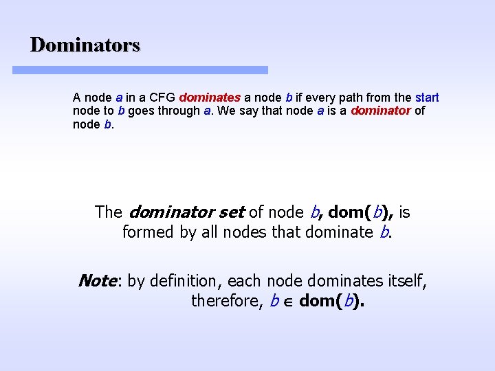
Dominators A node a in a CFG dominates a node b if every path from the start node to b goes through a. We say that node a is a dominator of node b. The dominator set of node b, dom(b), is formed by all nodes that dominate b. Note: by definition, each node dominates itself, therefore, b dom(b).

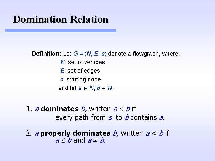
Domination Relation Definition: Let G = (N, E, s) denote a flowgraph, where: N: set of vertices E: set of edges s: starting node. and let a N, b N. 1. a dominates b, written a b if every path from s to b contains a. 2. a properly dominates b, written a < b if a b and a b.

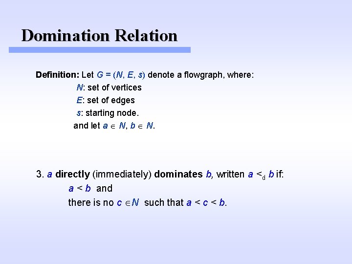
Domination Relation Definition: Let G = (N, E, s) denote a flowgraph, where: N: set of vertices E: set of edges s: starting node. and let a N, b N. 3. a directly (immediately) dominates b, written a <d b if: a < b and there is no c N such that a < c < b.

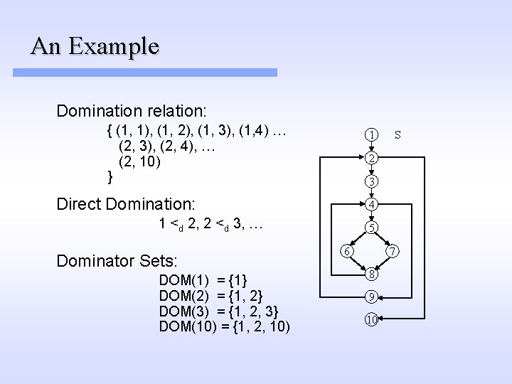
An Example Domination relation: { (1, 1), (1, 2), (1, 3), (1, 4) … (2, 3), (2, 4), … (2, 10) } 1 2 3 Direct Domination: 4 1 <d 2, 2 <d 3, … Dominator Sets: DOM(1) = {1} DOM(2) = {1, 2} DOM(3) = {1, 2, 3} DOM(10) = {1, 2, 10) S 5 6 7 8 9 10

Question Assume that node a is an immediate dominator of a node b. Is a necessarily an immediate predecessor of b in the flow graph?

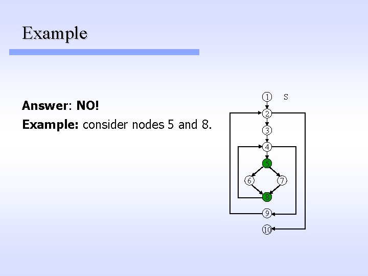
Example 1 Answer: NO! S 2 Example: consider nodes 5 and 8. 3 4 5 6 7 8 9 10

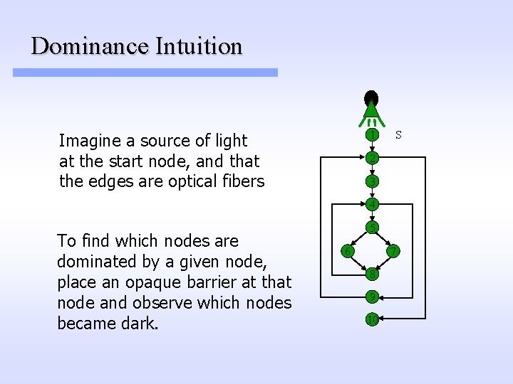
Dominance Intuition 1 Imagine a source of light at the start node, and that the edges are optical fibers S 2 3 4 To find which nodes are dominated by a given node, place an opaque barrier at that node and observe which nodes became dark. 5 6 7 8 9 10

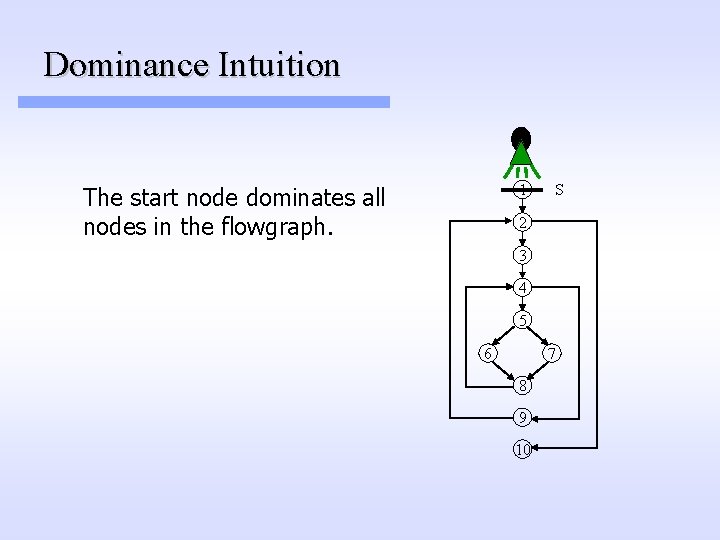
Dominance Intuition 1 The start node dominates all nodes in the flowgraph. S 2 3 4 5 6 7 8 9 10

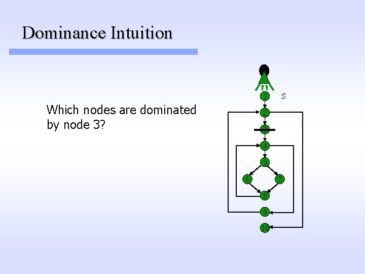
Dominance Intuition 1 Which nodes are dominated by node 3? S 2 3 4 5 6 7 8 9 10

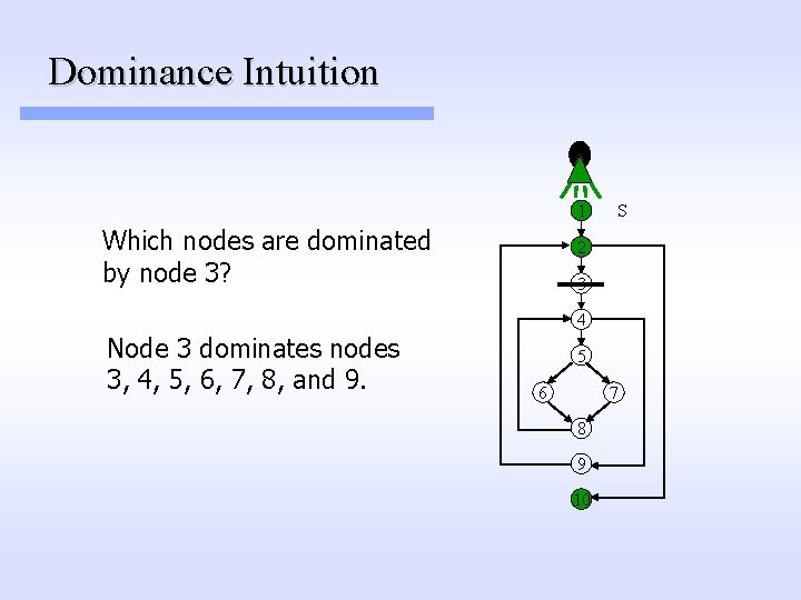
Dominance Intuition 1 Which nodes are dominated by node 3? S 2 3 4 Node 3 dominates nodes 3, 4, 5, 6, 7, 8, and 9. 5 6 7 8 9 10

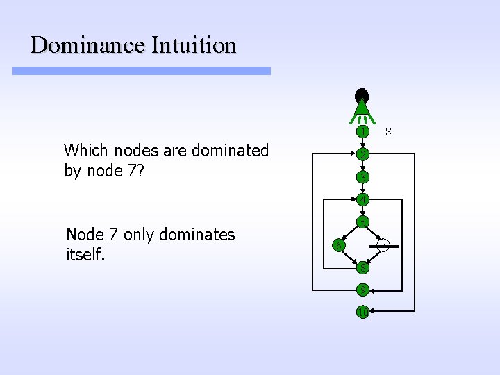
Dominance Intuition 1 Which nodes are dominated by node 7? S 2 3 4 Node 7 only dominates itself. 5 6 7 8 9 10

Dominator Tree A dominator tree is a useful way to represent the dominance relation. In a dominator tree the start node s is the root, and each node d dominates only its descendents in the tree. (Note a tree is possible since Dominance is reflexive and transitive)

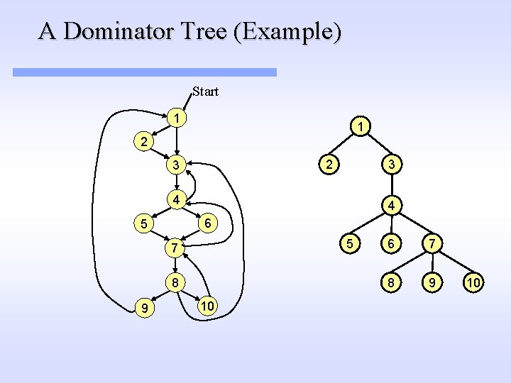
A Dominator Tree (Example) Start 1 1 2 3 4 4 6 5 5 7 8 9 10 6 7 8 9 10

Finding Loops Motivation: Programs spend most of the execution time in loops, therefore there is a larger payoff for optimizations that exploit loop structure. How do we identify loops in a flow graph? The goal is to create an uniform treatment for program loops written using different loop structures (e. g. while, for) and loops constructed out of goto’s. Basic idea: Use a general approach based on analyzing graph-theoretical properties of the CFG.

Definition def: A strongly-connected component (SCC) of flowgraph G = (N, E, s) is a subgraph G’ = (N’, E’, s’) in which there is a path from each node in N’ to every node in N’. A strongly-connected component G’ = (N’, E’, s’) is a loop with entry s’ if s’ dominates all nodes in N’.

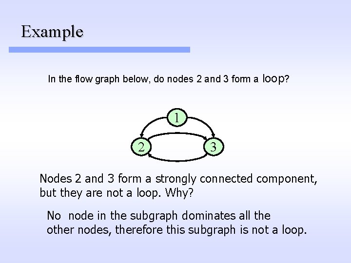
Example In the flow graph below, do nodes 2 and 3 form a loop? 1 2 3 Nodes 2 and 3 form a strongly connected component, but they are not a loop. Why? No node in the subgraph dominates all the other nodes, therefore this subgraph is not a loop.

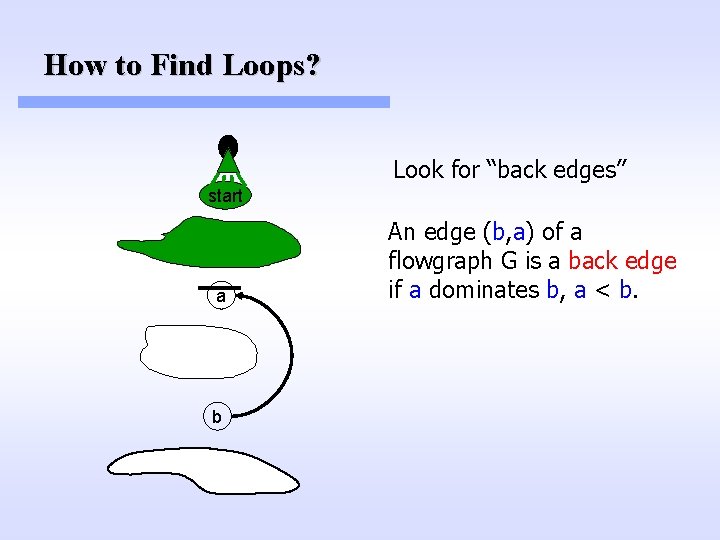
How to Find Loops? Look for “back edges” start a b An edge (b, a) of a flowgraph G is a back edge if a dominates b, a < b.

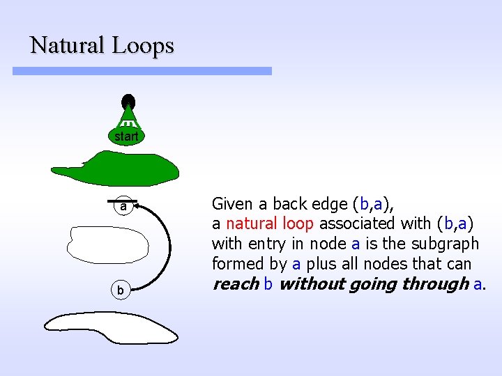
Natural Loops start a b Given a back edge (b, a), a natural loop associated with (b, a) with entry in node a is the subgraph formed by a plus all nodes that can reach b without going through a.

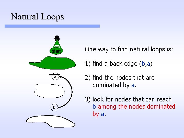
Natural Loops start One way to find natural loops is: 1) find a back edge (b, a) a b 2) find the nodes that are dominated by a. 3) look for nodes that can reach b among the nodes dominated by a.

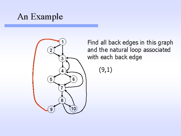
An Example Find all back edges in this graph and the natural loop associated with each back edge 1 2 3 (9, 1) 4 6 5 7 8 9 10

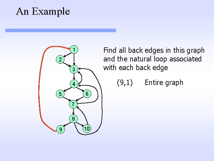
An Example Find all back edges in this graph and the natural loop associated with each back edge 1 2 3 (9, 1) 4 6 5 7 8 9 10 Entire graph

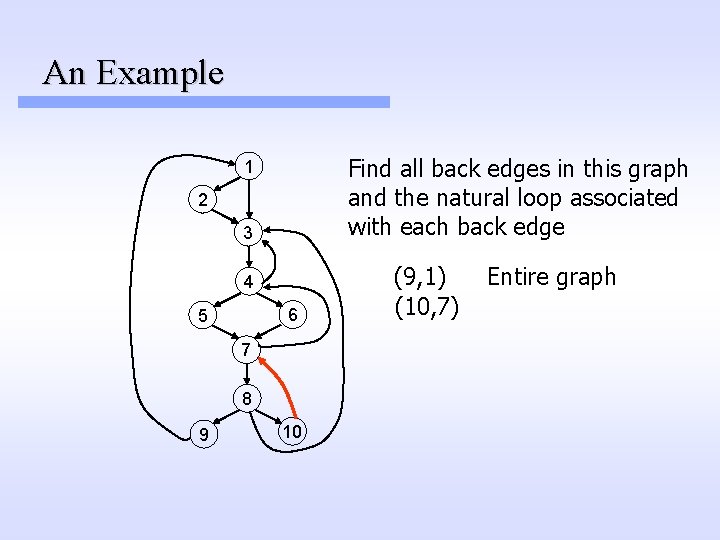
An Example Find all back edges in this graph and the natural loop associated with each back edge 1 2 3 4 6 5 7 8 9 10 (9, 1) (10, 7) Entire graph

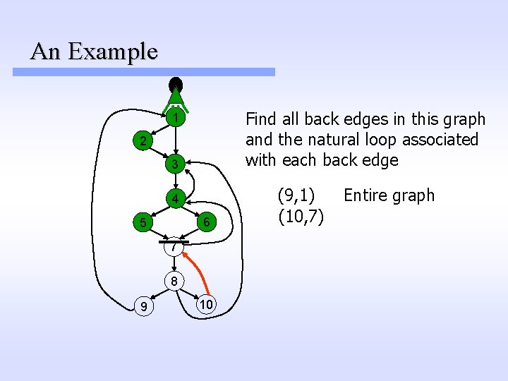
An Example Find all back edges in this graph and the natural loop associated with each back edge 1 2 3 4 6 5 7 8 9 10 (9, 1) (10, 7) Entire graph {7, 8, 10}

An Example Find all back edges in this graph and the natural loop associated with each back edge 1 2 3 4 6 5 7 8 9 10 (9, 1) (10, 7) (7, 4) Entire graph {7, 8, 10}

An Example Find all back edges in this graph and the natural loop associated with each back edge 1 2 3 4 6 5 7 8 9 10 (9, 1) (10, 7) (7, 4) Entire graph {7, 8, 10} {4, 5, 6, 7, 8, 10}

An Example Find all back edges in this graph and the natural loop associated with each back edge 1 2 3 4 6 5 7 8 9 10 (9, 1) (10, 7) (7, 4) (8, 3) Entire graph {7, 8, 10} {4, 5, 6, 7, 8, 10}

An Example Find all back edges in this graph and the natural loop associated with each back edge 1 2 3 4 6 5 7 8 9 10 (9, 1) (10, 7) (7, 4) (8, 3) Entire graph {7, 8, 10} {4, 5, 6, 7, 8, 10} {3, 4, 5, 6, 7, 8, 10}

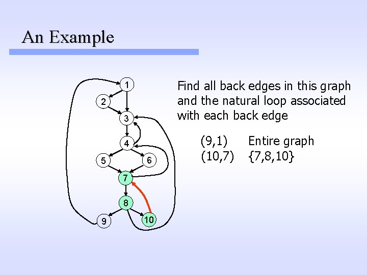
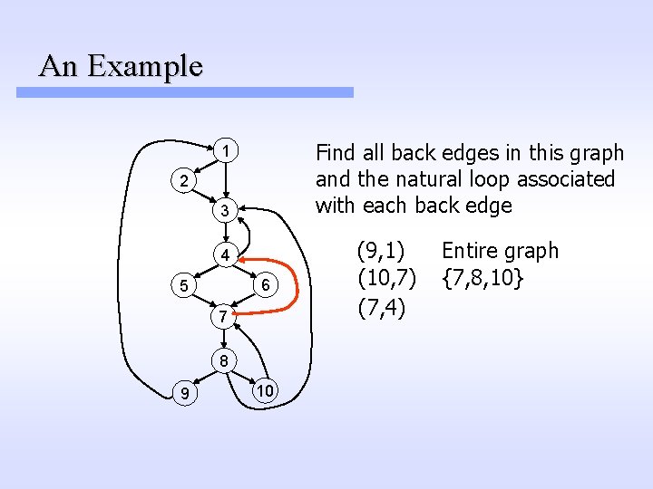
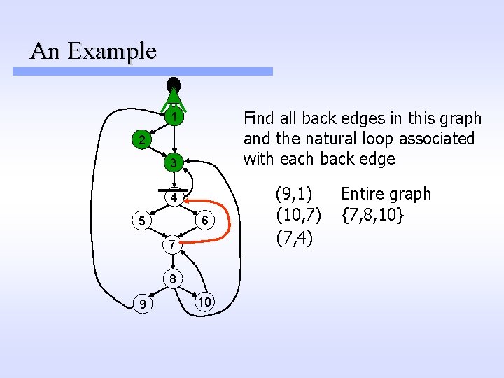
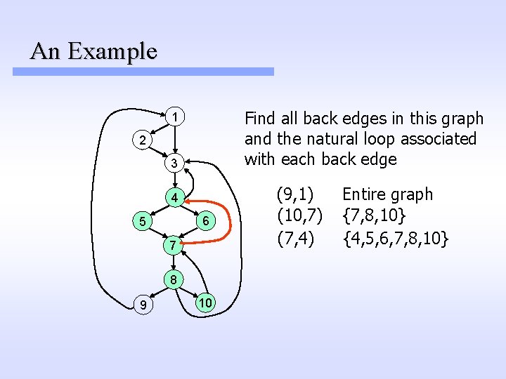
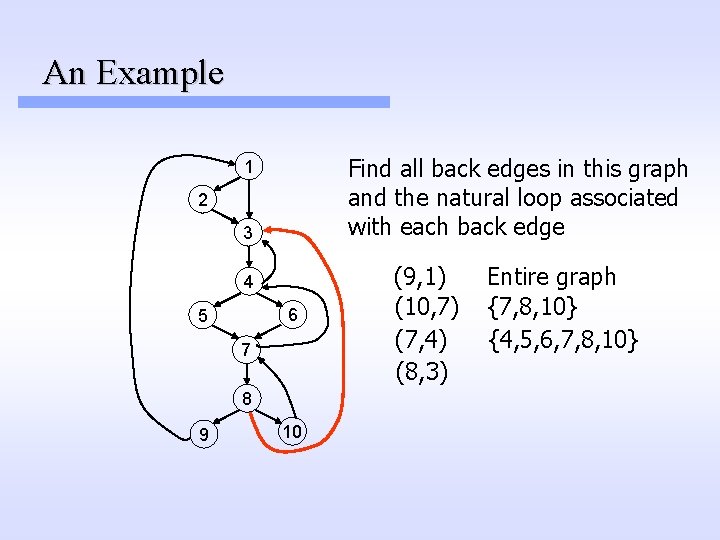
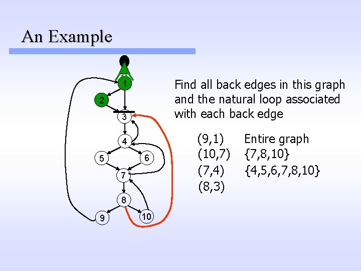
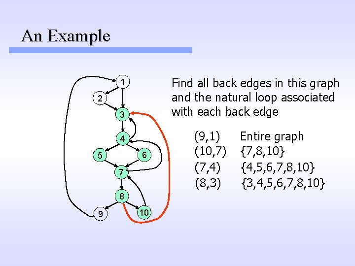
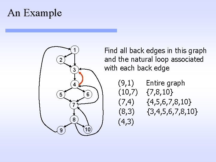
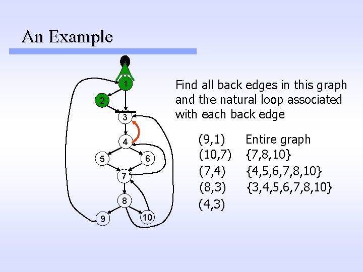
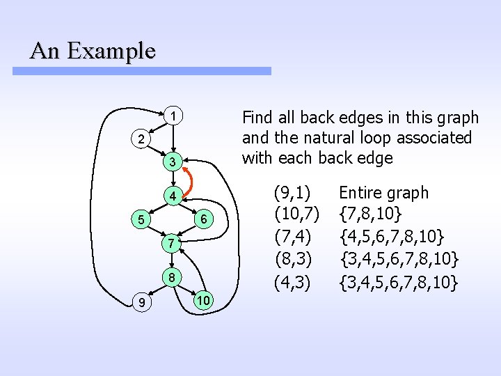
An Example Find all back edges in this graph and the natural loop associated with each back edge 1 2 3 4 6 5 7 8 9 10 (9, 1) (10, 7) (7, 4) (8, 3) (4, 3) Entire graph {7, 8, 10} {4, 5, 6, 7, 8, 10} {3, 4, 5, 6, 7, 8, 10}

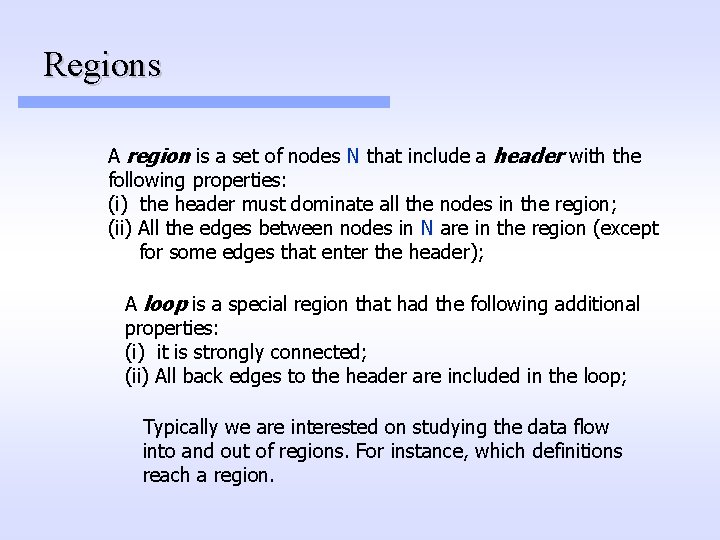
Regions A region is a set of nodes N that include a header with the following properties: (i) the header must dominate all the nodes in the region; (ii) All the edges between nodes in N are in the region (except for some edges that enter the header); A loop is a special region that had the following additional properties: (i) it is strongly connected; (ii) All back edges to the header are included in the loop; Typically we are interested on studying the data flow into and out of regions. For instance, which definitions reach a region.

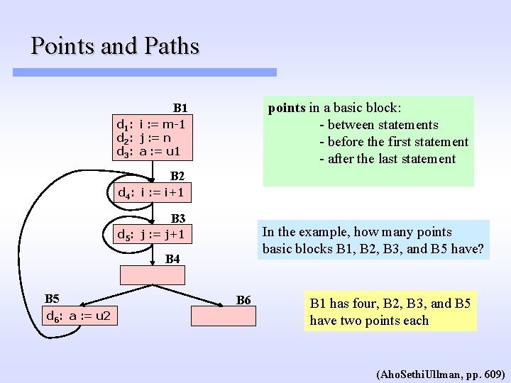
Points and Paths points in a basic block: - between statements - before the first statement - after the last statement B 1 d 1: i : = m-1 d 2: j : = n d 3: a : = u 1 B 2 d 4: i : = i+1 B 3 In the example, how many points basic blocks B 1, B 2, B 3, and B 5 have? d 5: j : = j+1 B 4 B 5 d 6: a : = u 2 B 6 B 1 has four, B 2, B 3, and B 5 have two points each (Aho. Sethi. Ullman, pp. 609)

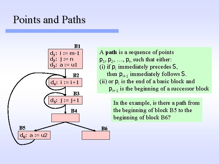
Points and Paths B 1 d 1: i : = m-1 d 2: j : = n d 3: a : = u 1 B 2 d 4: i : = i+1 B 3 A path is a sequence of points p 1, p 2, …, pn such that either: (i) if pi immediately precedes S, then pi+1 immediately follows S. (ii) or pi is the end of a basic block and pi+1 is the beginning of a successor block d 5: j : = j+1 In the example, is there a path from the beginning of block B 5 to the beginning of block B 6? B 4 B 5 d 6: a : = u 2 B 6

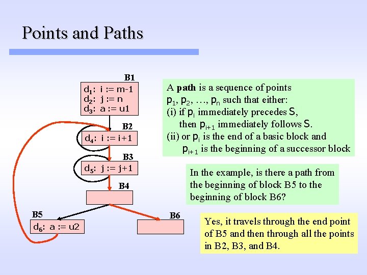
Points and Paths B 1 d 1: i : = m-1 d 2: j : = n d 3: a : = u 1 B 2 d 4: i : = i+1 B 3 A path is a sequence of points p 1, p 2, …, pn such that either: (i) if pi immediately precedes S, then pi+1 immediately follows S. (ii) or pi is the end of a basic block and pi+1 is the beginning of a successor block d 5: j : = j+1 In the example, is there a path from the beginning of block B 5 to the beginning of block B 6? B 4 B 5 d 6: a : = u 2 B 6 Yes, it travels through the end point of B 5 and then through all the points in B 2, B 3, and B 4.

Global Dataflow Analysis Motivation We need to know variable def and use information between basic blocks for: – constant folding – dead-code elimination – redundant computation elimination – code motion – induction variable elimination – build data dependence graph (DDG)

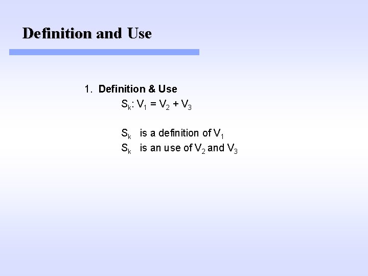
Definition and Use 1. Definition & Use Sk: V 1 = V 2 + V 3 Sk is a definition of V 1 Sk is an use of V 2 and V 3

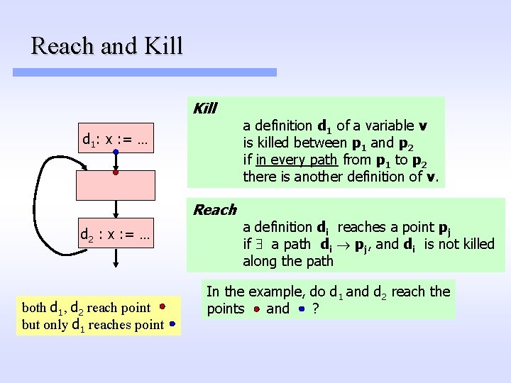
Reach and Kill d 1: x : = … Reach d 2 : x : = … both d 1, d 2 reach point but only d 1 reaches point a definition d 1 of a variable v is killed between p 1 and p 2 if in every path from p 1 to p 2 there is another definition of v. a definition di reaches a point pj if a path di pj, and di is not killed along the path In the example, do d 1 and d 2 reach the points and ?

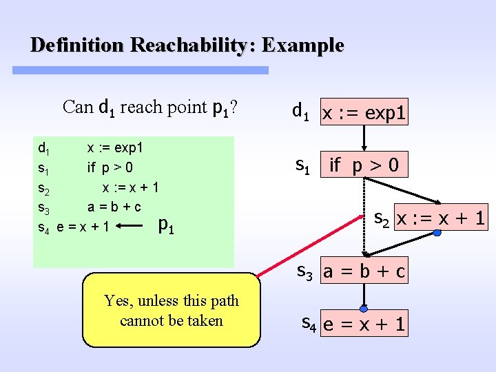
Definition Reachability: Example Can d 1 reach point p 1? d 1 x : = exp 1 s 1 if p > 0 s 2 x : = x + 1 s 3 a=b+c p 1 s 4 e = x + 1 d 1 x : = exp 1 s 1 if p > 0 s 2 x : = x + 1 s 3 a = b + c Yes, unless this path cannot be taken s 4 e = x + 1

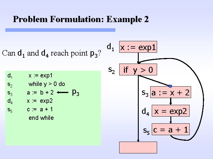
Problem Formulation: Example 2 Can d 1 and d 4 reach point p 3? d 1 s 2 s 3 d 4 s 5 x : = exp 1 while y > 0 do a : = b + 2 x : = exp 2 c : = a + 1 end while d 1 x : = exp 1 s 2 p 3 if y > 0 s 3 a : = x + 2 d 4 x = exp 2 s 5 c = a + 1

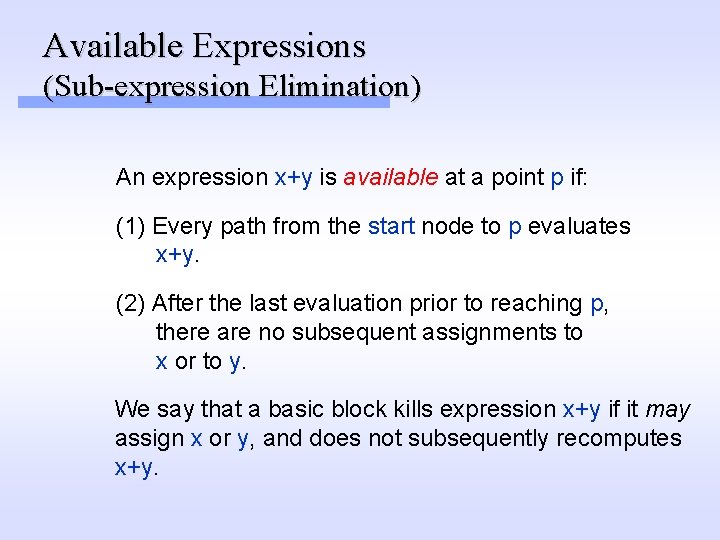
Available Expressions (Sub-expression Elimination) An expression x+y is available at a point p if: (1) Every path from the start node to p evaluates x+y. (2) After the last evaluation prior to reaching p, there are no subsequent assignments to x or to y. We say that a basic block kills expression x+y if it may assign x or y, and does not subsequently recomputes x+y.

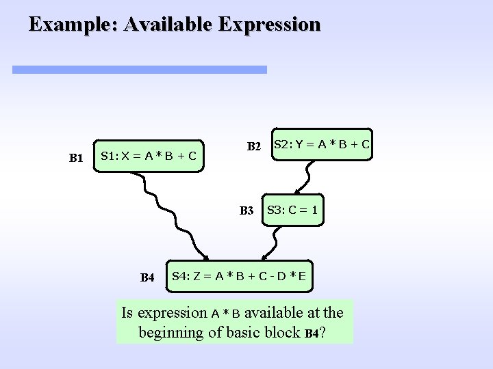
Example: Available Expression B 1 S 1: X = A * B + C B 2 B 3 B 4 S 2: Y = A * B + C S 3: C = 1 S 4: Z = A * B + C - D * E Is expression A * B available at the beginning of basic block B 4?

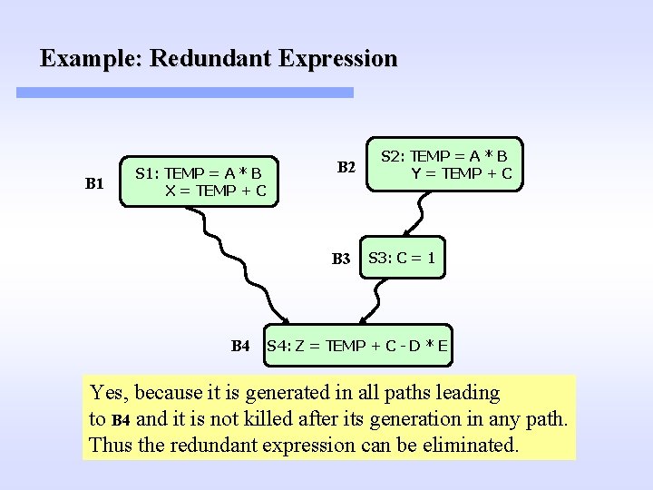
Example: Redundant Expression B 1 S 1: TEMP = A * B X = TEMP + C B 2 B 3 B 4 S 2: TEMP = A * B Y = TEMP + C S 3: C = 1 S 4: Z = TEMP + C - D * E Yes, because it is generated in all paths leading to B 4 and it is not killed after its generation in any path. Thus the redundant expression can be eliminated.

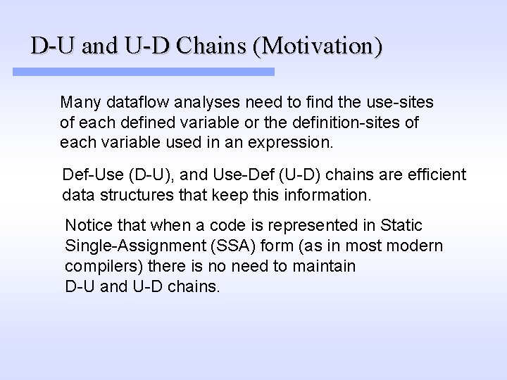
D-U and U-D Chains (Motivation) Many dataflow analyses need to find the use-sites of each defined variable or the definition-sites of each variable used in an expression. Def-Use (D-U), and Use-Def (U-D) chains are efficient data structures that keep this information. Notice that when a code is represented in Static Single-Assignment (SSA) form (as in most modern compilers) there is no need to maintain D-U and U-D chains.

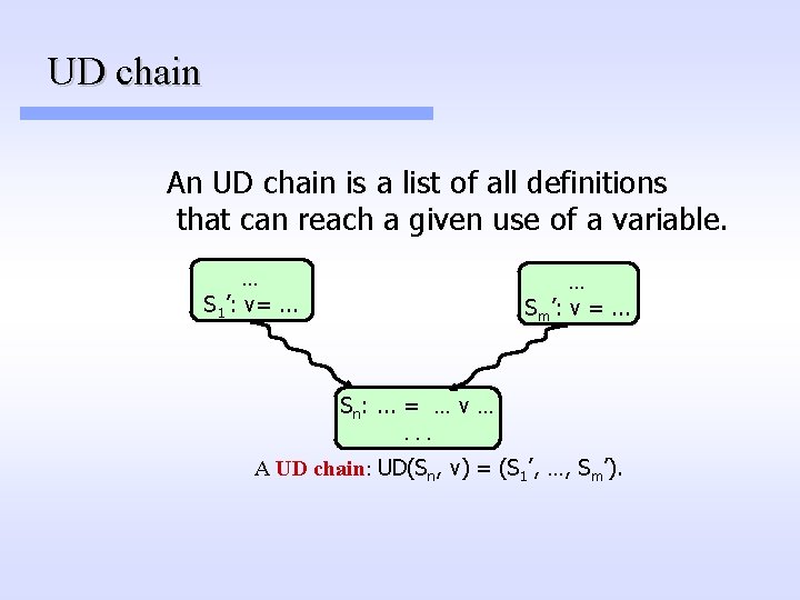
UD chain An UD chain is a list of all definitions that can reach a given use of a variable. . S 1’: v=. . . Sm’: v =. . . Sn: . . . = … v …. . . A UD chain: UD(Sn, v) = (S 1’, …, Sm’).

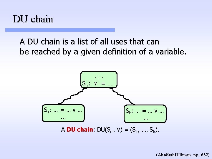
DU chain A DU chain is a list of all uses that can be reached by a given definition of a variable. . Sn’: v = … S 1 : … = … v …. . . Sk : … = … v …. . . A DU chain: DU(Sn’, v) = (S 1, …, Sk). (Aho. Sethi. Ullman, pp. 632)

Reaching Definitions Problem Statement: Determine the set of definitions reaching a point in a program. To solve this problem we must take into consideration the data-flow and the control flow in the program. A common method to solve such a problem is to create a set of data-flow equations.

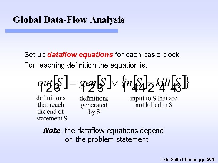
Global Data-Flow Analysis Set up dataflow equations for each basic block. For reaching definition the equation is: Note: the dataflow equations depend on the problem statement (Aho. Sethi. Ullman, pp. 608)

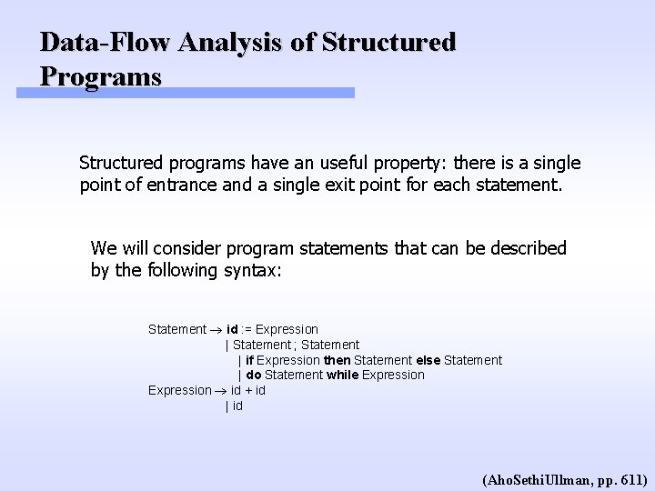
Data-Flow Analysis of Structured Programs Structured programs have an useful property: there is a single point of entrance and a single exit point for each statement. We will consider program statements that can be described by the following syntax: Statement id : = Expression | Statement ; Statement | if Expression then Statement else Statement | do Statement while Expression id + id | id (Aho. Sethi. Ullman, pp. 611)

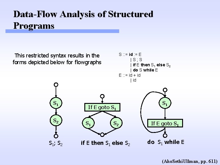
Data-Flow Analysis of Structured Programs This restricted syntax results in the forms depicted below for flowgraphs S 1 S 2 S 1 ; S 2 S : : = id : = E |S; S | if E then S 1 else S 2 | do S while E E : : = id + id | id If E goto S 1 S 2 if E then S 1 else S 2 S 1 If E goto S 1 do S 1 while E (Aho. Sethi. Ullman, pp. 611)

Data-flow equations for reaching definitions Dataflow Equations for Reaching Definition gen[S] = {d} S d : a : = b + c kill [S] = Def(a) - {d} S S 1 gen [S] = gen [S 2] (gen [S 1] - kill [S 2]) S 2 kill [S] = kill [S 2] (kill [S 1] - gen [S 2]) gen [S] = gen [S 1] gen [S 2] S S S 1 S 2 S 1 kill [S] = kill [S 1] kill [S 2] gen [S] = gen [S 1] kill [S] = kill [S 1] (Aho. Sethi. Ullman, pp. 612)

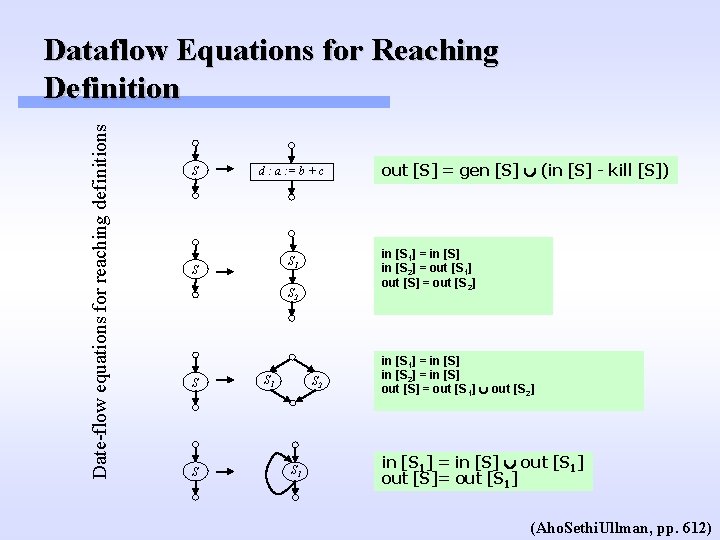
Date-flow equations for reaching definitions Dataflow Equations for Reaching Definition S d : a : = b + c in [S 1] = in [S] in [S 2] = out [S 1] out [S] = out [S 2] S 1 S S 2 S S S 1 S 2 S 1 out [S] = gen [S] (in [S] - kill [S]) in [S 1] = in [S] in [S 2] = in [S] out [S] = out [S 1] out [S 2] in [S 1] = in [S] out [S 1] out [S]= out [S 1] (Aho. Sethi. Ullman, pp. 612)

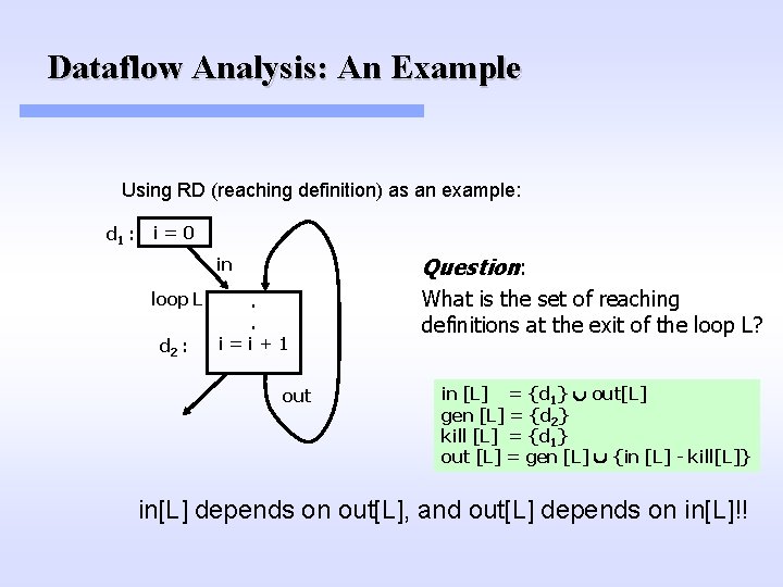
Dataflow Analysis: An Example Using RD (reaching definition) as an example: d 1 : i=0 loop L d 2 : in Question: . . i=i+1 What is the set of reaching definitions at the exit of the loop L? out in [L] = {d 1} out[L] gen [L] = {d 2} kill [L] = {d 1} out [L] = gen [L] {in [L] - kill[L]} in[L] depends on out[L], and out[L] depends on in[L]!!

Solution? Initialization out[L] = First iteration in[L] = {d 1} out[L] = {d 1} out[L] = gen [L] (in [L] - kill [L]) = {d 2} ({d 1} - {d 1}) = {d 2} d 1 : i=0 in loop L d 2 : . . i=i+1 out in [L] = {d 1} out[L] gen [L] = {d 2} kill [L] = {d 1} out [L] = gen [L] {in [L] - kill[L]}

Solution d 1 : i=0 First iteration out[L] = {d 2} Second iteration in[L] = {d 1} out[L] = {d 1, d 2} out[L] = gen [L] (in [L] - kill [L]) = {d 2} {{d 1, d 2} - {d 1}} = {d 2} We reached the fixed point! in loop L d 2 : . . i=i+1 out in [L] = {d 1} out[L] gen [L] = {d 2} kill [L] = {d 1} out [L] = gen [L] {in [L] - kill[L]}

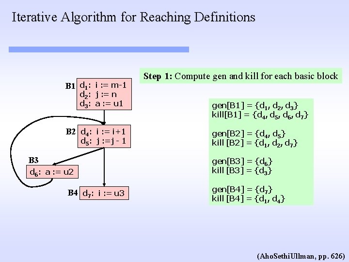
Iterative Algorithm for Reaching Definitions B 1 d 1: i : = m-1 d 2: j : = n d 3: a : = u 1 B 2 d 4: i : = i+1 d 5: j : =j - 1 B 3 d 6: a : = u 2 B 4 d 7: i : = u 3 Step 1: Compute gen and kill for each basic block gen[B 1] = {d 1, d 2, d 3} kill[B 1] = {d 4, d 5, d 6, d 7} gen[B 2] = {d 4, d 5} kill [B 2] = {d 1, d 2, d 7} gen[B 3] = {d 6} kill [B 3] = {d 3} gen[B 4] = {d 7} kill [B 4] = {d 1, d 4} (Aho. Sethi. Ullman, pp. 626)

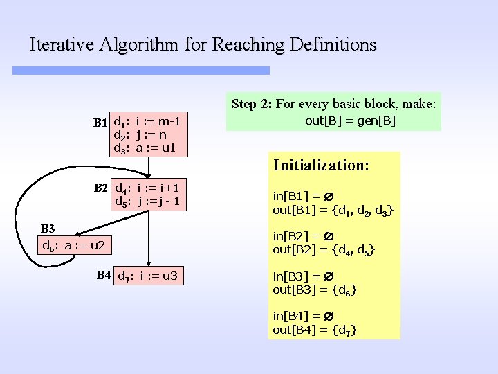
Iterative Algorithm for Reaching Definitions Step 2: For every basic block, make: B 1 d 1: i : = m-1 d 2: j : = n d 3: a : = u 1 B 2 d 4: i : = i+1 d 5: j : =j - 1 B 3 d 6: a : = u 2 B 4 d 7: i : = u 3 out[B] = gen[B] Initialization: in[B 1] = out[B 1] = {d 1, d 2, d 3} in[B 2] = out[B 2] = {d 4, d 5} in[B 3] = out[B 3] = {d 6} in[B 4] = out[B 4] = {d 7}

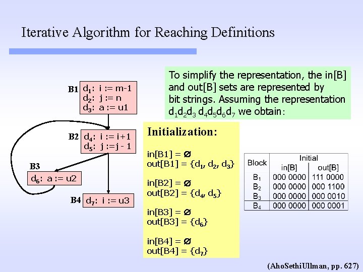
Iterative Algorithm for Reaching Definitions B 1 d 1: i : = m-1 d 2: j : = n d 3: a : = u 1 B 2 d 4: i : = i+1 d 5: j : =j - 1 B 3 d 6: a : = u 2 B 4 d 7: i : = u 3 To simplify the representation, the in[B] and out[B] sets are represented by bit strings. Assuming the representation d 1 d 2 d 3 d 4 d 5 d 6 d 7 we obtain: Initialization: in[B 1] = out[B 1] = {d 1, d 2, d 3} in[B 2] = out[B 2] = {d 4, d 5} in[B 3] = out[B 3] = {d 6} in[B 4] = out[B 4] = {d 7} (Aho. Sethi. Ullman, pp. 627)

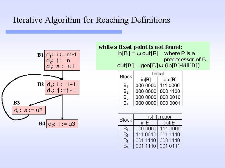
Iterative Algorithm for Reaching Definitions while a fixed point is not found: B 1 d 1: i : = m-1 d 2: j : = n d 3: a : = u 1 in[B] = out[P] where P is a predecessor of B out[B] = gen[B] (in[B]-kill[B]) B 2 d 4: i : = i+1 d 5: j : =j - 1 B 3 d 6: a : = u 2 B 4 d 7: i : = u 3 Block B 1 B 2 B 3 B 4 First Iteration in[B] out[B] 0000 111 0010 001 1110 000 1110 001 0111

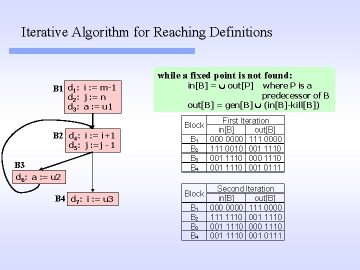
Iterative Algorithm for Reaching Definitions while a fixed point is not found: B 1 d 1: i : = m-1 d 2: j : = n d 3: a : = u 1 in[B] = out[P] where P is a predecessor of B out[B] = gen[B] (in[B]-kill[B]) Block B 2 d 4: i : = i+1 d 5: j : =j - 1 B 3 d 6: a : = u 2 B 4 d 7: i : = u 3 B 1 B 2 B 3 B 4 Block B 1 B 2 B 3 B 4 First Iteration in[B] out[B] 0000 111 0010 001 1110 000 1110 001 0111 Second Iteration in[B] out[B] 0000 1110 001 1110 000 1110 001 0111

Algorithm Convergence Intuitively we can observe that the algorithm converges to a fix point because the out[B] set never decreases in size It can be shown that an upper bound on the number of iterations required to reach a fix point is the number of nodes in the control flow graph. Intuitively, if a definition reaches a point, it can reach the point through a cycle free path, and no cycle free path can be longer than the number of nodes in the graph. Empirical evidence suggests that for real programs the number of iterations required to reach a fix point is typically less then five. (Aho. Sethi. Ullman, pp. 626)

Conclusions l Basic Blocks – Group of statements that execute atomically – Leader algorithm – finds basic blocks in MIR Control Flow Graphs – model the control dependencies between basic blocks l Dominance relations l – Shows control dependencies between BBs – Used to determine natural loops – Points, Paths and Regions used to reason about data flow l Data flow analysis – Local – how data flows through small region like Basic Blocks or Regions – Global – how data flows through different control paths – Iterative data flow analysis • General – can solve many different flow analysis • Uses underlying “generic” lattice structure

References and Copyright l Copyright – José Nelson Amaral – Alberta CS Dept. CMPUT 680 - Winter 2001 l References – Muchnick – Chapter 7 – Aho - Chapter 10 – Appel - section 8. 2, chapter 10 (page 218), chapter 18 (pp 408 -418)