Lecture 6 Optimization CS 109 B Data Science

Lecture 6: Optimization CS 109 B Data Science 2 Pavlos Protopapas and Mark Glickman

Outline Optimization • • • Challenges in Optimization Momentum Adaptive Learning Rate Parameter Initialization Batch Normalization CS 109 B, PROTOPAPAS, GLICKMAN 2

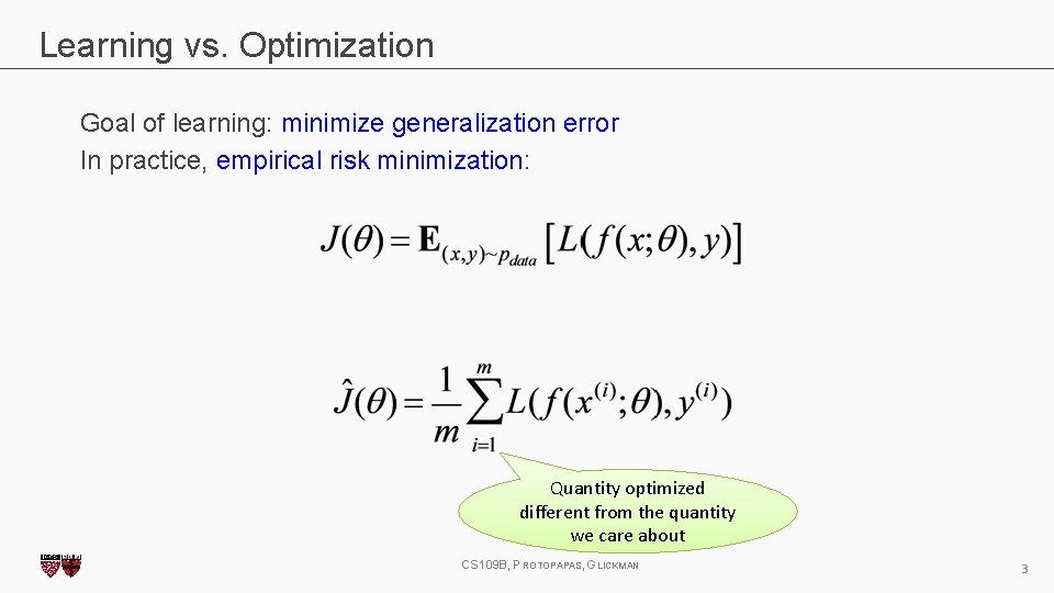
Learning vs. Optimization Goal of learning: minimize generalization error In practice, empirical risk minimization: Quantity optimized different from the quantity we care about CS 109 B, PROTOPAPAS, GLICKMAN 3

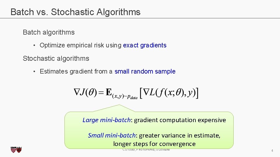
Batch vs. Stochastic Algorithms Batch algorithms • Optimize empirical risk using exact gradients Stochastic algorithms • Estimates gradient from a small random sample Large mini-batch: gradient computation expensive Small mini-batch: greater variance in estimate, longer steps for convergence CS 109 B, PROTOPAPAS, GLICKMAN 4

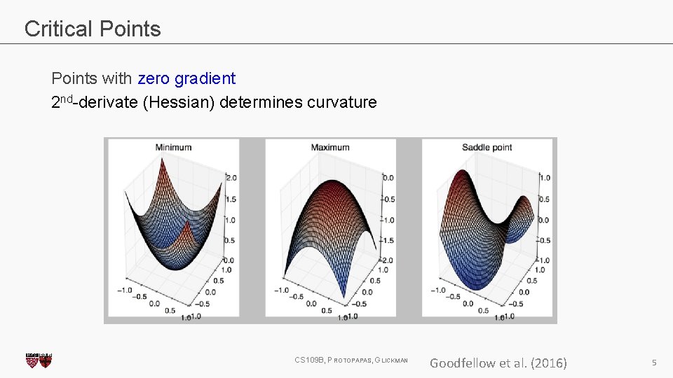
Critical Points with zero gradient 2 nd-derivate (Hessian) determines curvature CS 109 B, PROTOPAPAS, GLICKMAN Goodfellow et al. (2016) 5

Stochastic Gradient Descent Take small steps in direction of negative gradient Sample m examples from training set and compute: Update parameters: In practice: shuffle training set once and pass through multiple times CS 109 B, PROTOPAPAS, GLICKMAN 6

Outline Optimization • • • Challenges in Optimization Momentum Adaptive Learning Rate Parameter Initialization Batch Normalization CS 109 B, PROTOPAPAS, GLICKMAN 7

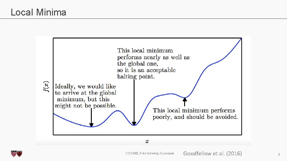
Local Minima CS 109 B, PROTOPAPAS, GLICKMAN Goodfellow et al. (2016) 8

Local Minima Old view: local minima is major problem in neural network training Recent view: • For sufficiently large neural networks, most local minima incur low cost • Not important to find true global minimum CS 109 B, PROTOPAPAS, GLICKMAN 9

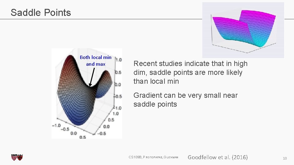
Saddle Points Both local min and max Recent studies indicate that in high dim, saddle points are more likely than local min Gradient can be very small near saddle points CS 109 B, PROTOPAPAS, GLICKMAN Goodfellow et al. (2016) 10

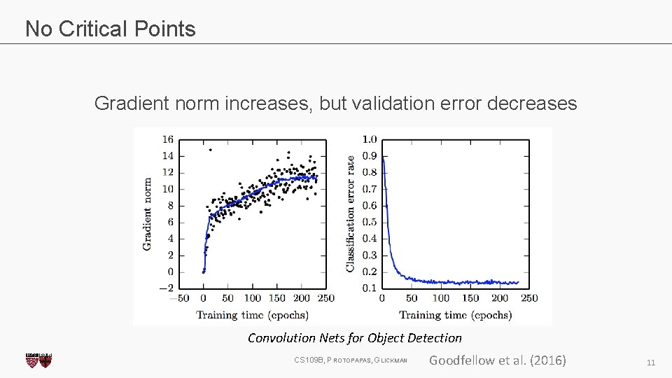
No Critical Points Gradient norm increases, but validation error decreases Convolution Nets for Object Detection CS 109 B, PROTOPAPAS, GLICKMAN Goodfellow et al. (2016) 11

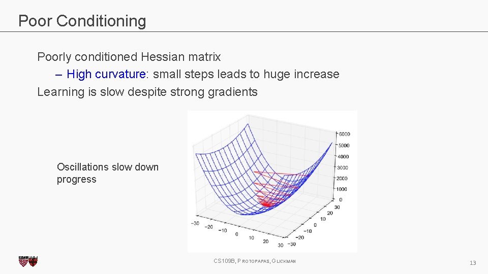
Poor Conditioning Poorly conditioned Hessian matrix – High curvature: small steps leads to huge increase Learning is slow despite strong gradients Oscillations slow down progress CS 109 B, PROTOPAPAS, GLICKMAN 13

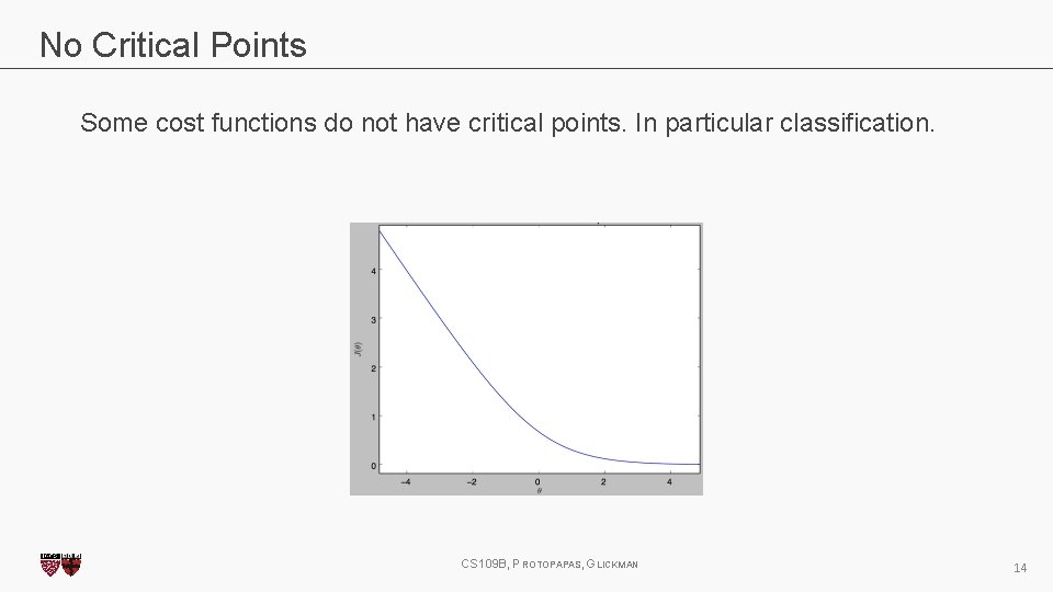
No Critical Points Some cost functions do not have critical points. In particular classification. CS 109 B, PROTOPAPAS, GLICKMAN 14

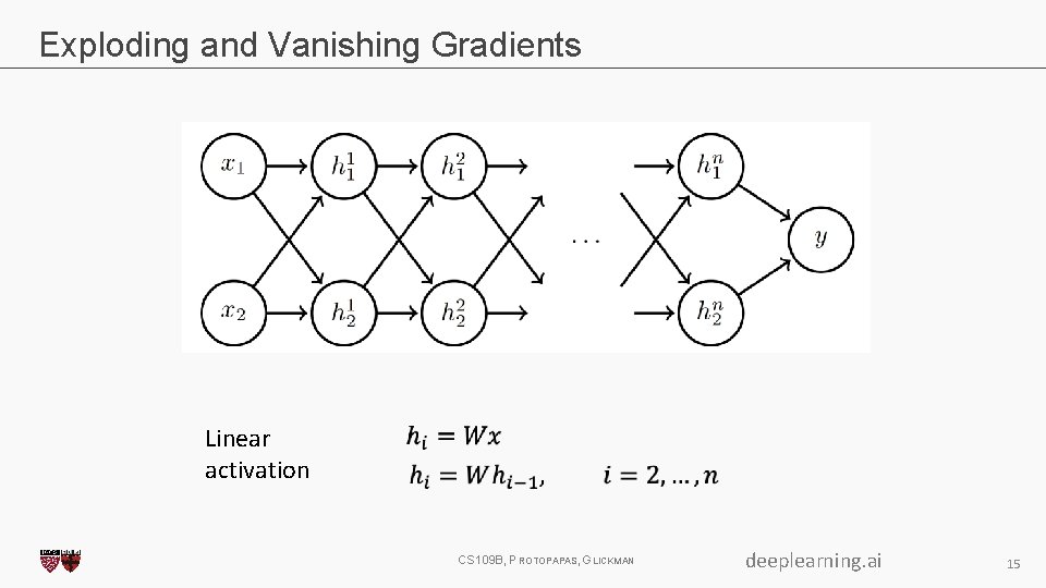
Exploding and Vanishing Gradients Linear activation CS 109 B, PROTOPAPAS, GLICKMAN deeplearning. ai 15

Exploding and Vanishing Gradients CS 109 B, PROTOPAPAS, GLICKMAN 16

Exploding and Vanishing Gradients Explodes! Vanishes! CS 109 B, PROTOPAPAS, GLICKMAN 17

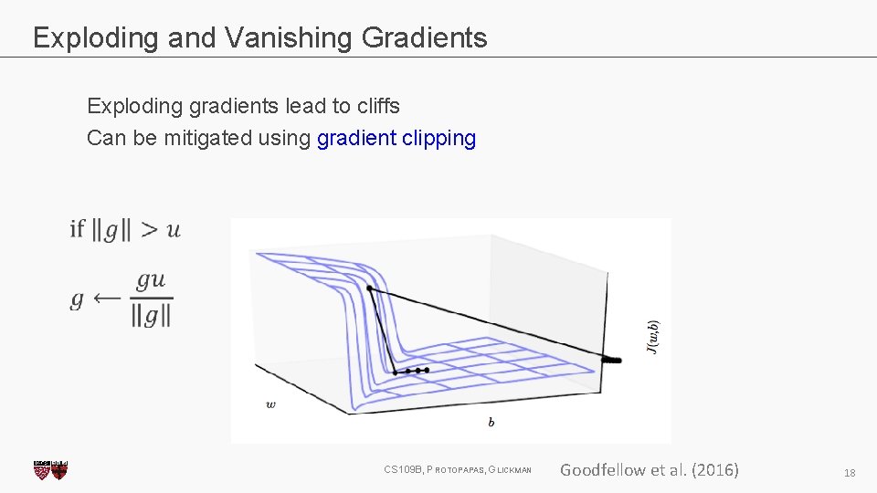
Exploding and Vanishing Gradients Exploding gradients lead to cliffs Can be mitigated using gradient clipping CS 109 B, PROTOPAPAS, GLICKMAN Goodfellow et al. (2016) 18

Outline Optimization • • • Challenges in Optimization Momentum Adaptive Learning Rate Parameter Initialization Batch Normalization CS 109 B, PROTOPAPAS, GLICKMAN 19

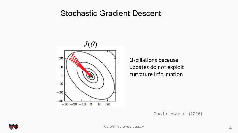
Stochastic Gradient Descent Oscillations because updates do not exploit curvature information Goodfellow et al. (2016) CS 109 B, PROTOPAPAS, GLICKMAN 20

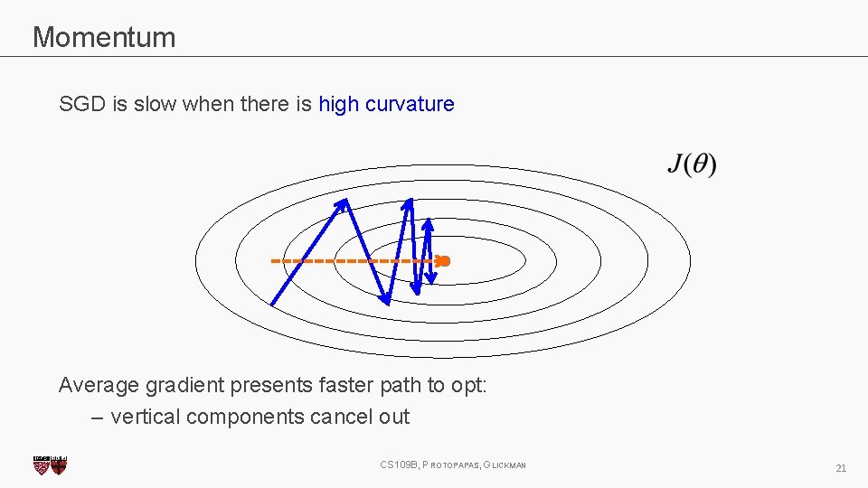
Momentum SGD is slow when there is high curvature Average gradient presents faster path to opt: – vertical components cancel out CS 109 B, PROTOPAPAS, GLICKMAN 21

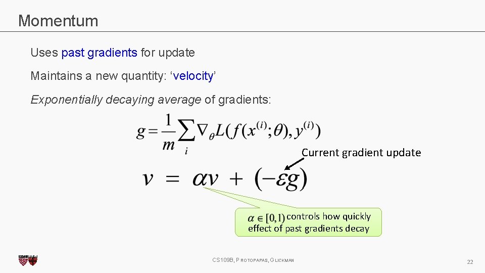
Momentum Uses past gradients for update Maintains a new quantity: ‘velocity’ Exponentially decaying average of gradients: Current gradient update controls how quickly effect of past gradients decay CS 109 B, PROTOPAPAS, GLICKMAN 22

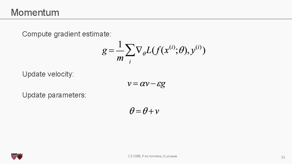
Momentum Compute gradient estimate: Update velocity: Update parameters: CS 109 B, PROTOPAPAS, GLICKMAN 23

Momentum Damped oscillations: gradients in opposite directions get cancelled out CS 109 B, PROTOPAPAS, GLICKMAN Goodfellow et al. (2016) 24

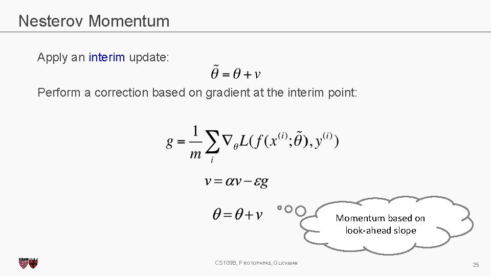
Nesterov Momentum Apply an interim update: Perform a correction based on gradient at the interim point: Momentum based on look-ahead slope CS 109 B, PROTOPAPAS, GLICKMAN 25

26

Outline Optimization • • • Challenges in Optimization Momentum Adaptive Learning Rate Parameter Initialization Batch Normalization CS 109 B, PROTOPAPAS, GLICKMAN 27

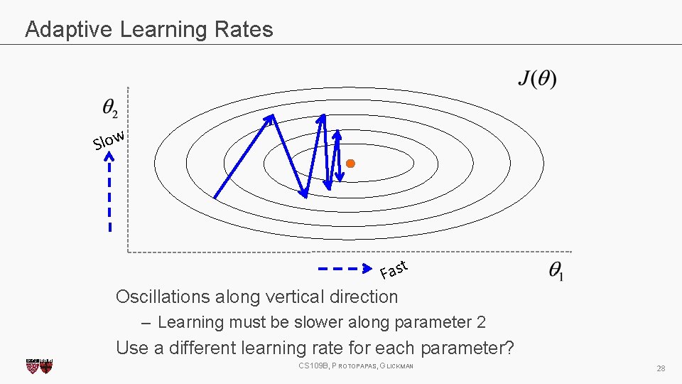
Adaptive Learning Rates Slow t Fas Oscillations along vertical direction – Learning must be slower along parameter 2 Use a different learning rate for each parameter? CS 109 B, PROTOPAPAS, GLICKMAN 28

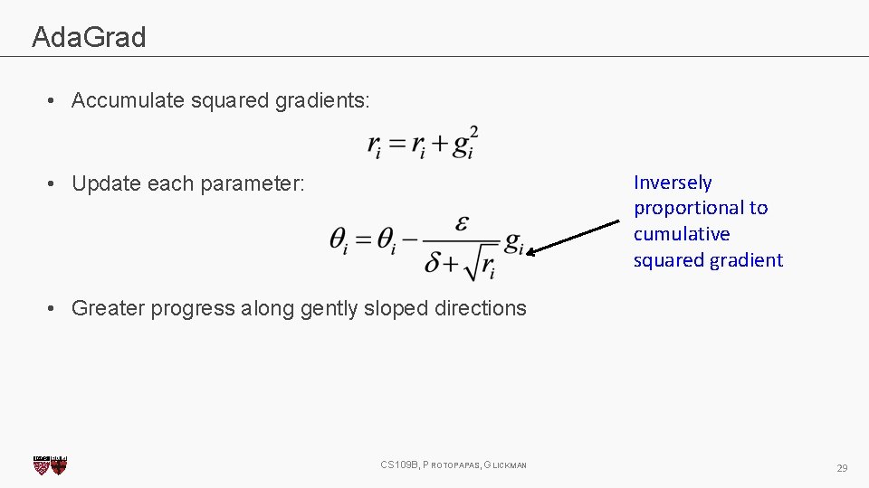
Ada. Grad • Accumulate squared gradients: Inversely proportional to cumulative squared gradient • Update each parameter: • Greater progress along gently sloped directions CS 109 B, PROTOPAPAS, GLICKMAN 29

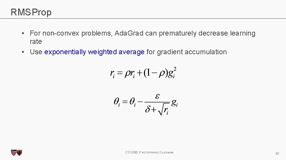
RMSProp • For non-convex problems, Ada. Grad can prematurely decrease learning rate • Use exponentially weighted average for gradient accumulation CS 109 B, PROTOPAPAS, GLICKMAN 30

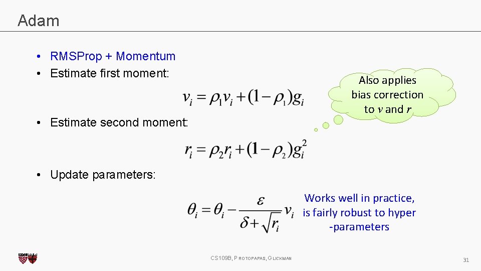
Adam • RMSProp + Momentum • Estimate first moment: Also applies bias correction to v and r • Estimate second moment: • Update parameters: Works well in practice, is fairly robust to hyper -parameters CS 109 B, PROTOPAPAS, GLICKMAN 31

Outline Optimization • • • Challenges in Optimization Momentum Adaptive Learning Rate Parameter Initialization Batch Normalization CS 109 B, PROTOPAPAS, GLICKMAN 32

Parameter Initialization • Goal: break symmetry between units • so that each unit computes a different function • Initialize all weights (not biases) randomly • Gaussian or uniform distribution • Scale of initialization? • Large -> grad explosion, Small -> grad vanishing CS 109 B, PROTOPAPAS, GLICKMAN 33

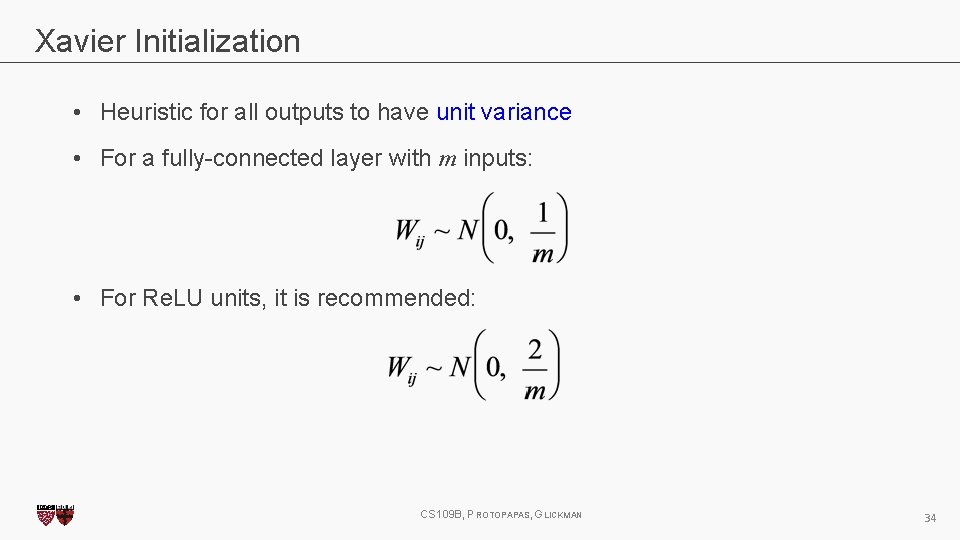
Xavier Initialization • Heuristic for all outputs to have unit variance • For a fully-connected layer with m inputs: • For Re. LU units, it is recommended: CS 109 B, PROTOPAPAS, GLICKMAN 34

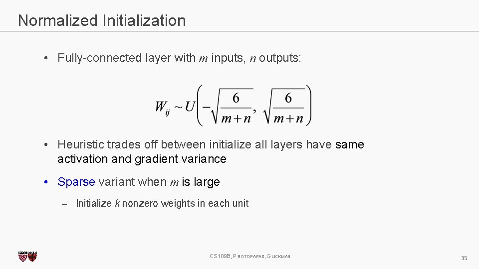
Normalized Initialization • Fully-connected layer with m inputs, n outputs: • Heuristic trades off between initialize all layers have same activation and gradient variance • Sparse variant when m is large – Initialize k nonzero weights in each unit CS 109 B, PROTOPAPAS, GLICKMAN 35

37

Outline Challenges in Optimization Momentum Adaptive Learning Rate Parameter Initialization Batch Normalization CS 109 B, PROTOPAPAS, GLICKMAN 38

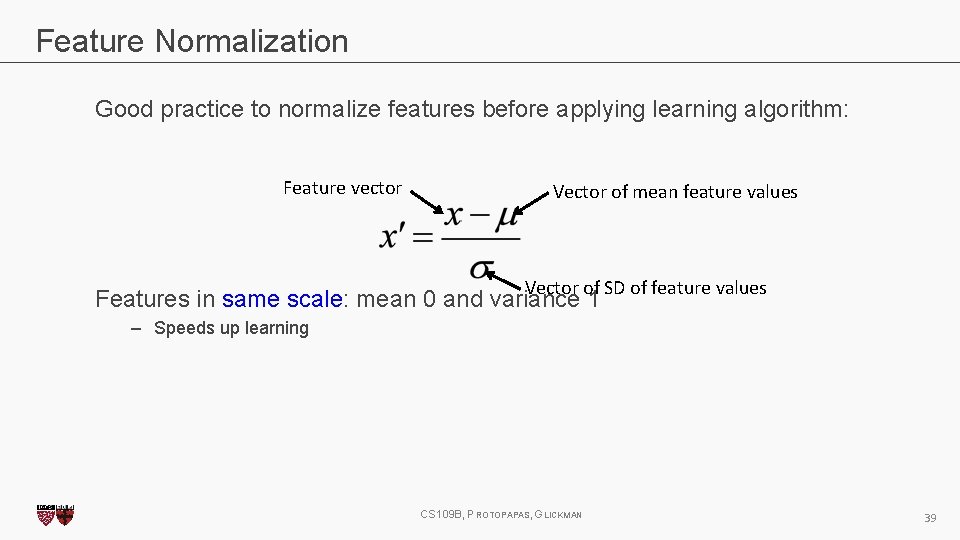
Feature Normalization Good practice to normalize features before applying learning algorithm: Feature vector Vector of mean feature values Vector of SD of feature values Features in same scale: mean 0 and variance 1 – Speeds up learning CS 109 B, PROTOPAPAS, GLICKMAN 39

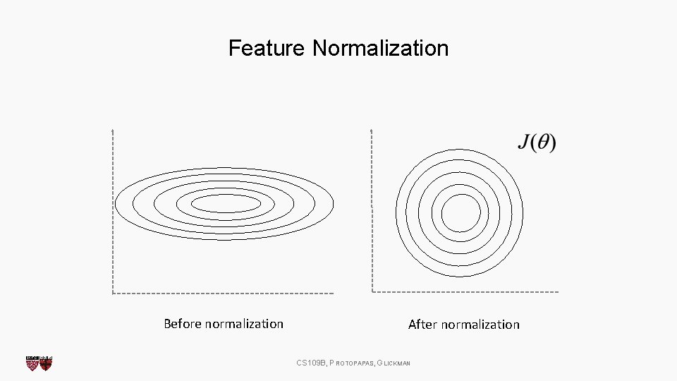
Feature Normalization Before normalization After normalization CS 109 B, PROTOPAPAS, GLICKMAN

Internal Covariance Shift Each hidden layer changes distribution of inputs to next layer: slows down learning Normalize inputs to layer 2 … Normalize CS 109 B, PROTOPAPAS, GLICKMANinputs to layer n 41

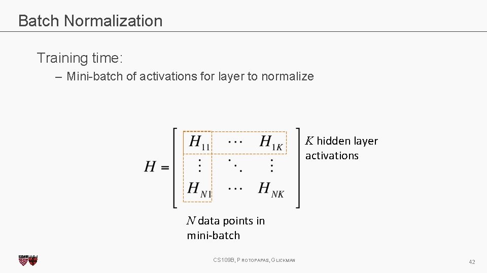
Batch Normalization Training time: – Mini-batch of activations for layer to normalize K hidden layer activations N data points in mini-batch CS 109 B, PROTOPAPAS, GLICKMAN 42

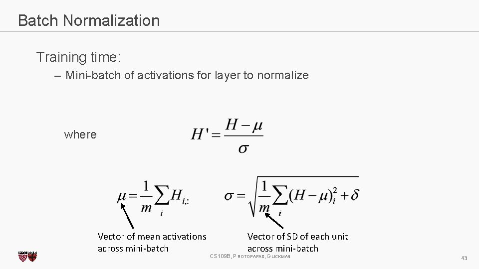
Batch Normalization Training time: – Mini-batch of activations for layer to normalize where Vector of mean activations across mini-batch Vector of SD of each unit across mini-batch CS 109 B, PROTOPAPAS, GLICKMAN 43

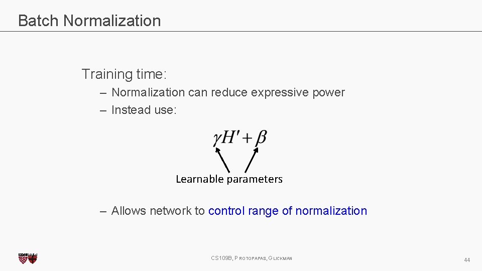
Batch Normalization Training time: – Normalization can reduce expressive power – Instead use: Learnable parameters – Allows network to control range of normalization CS 109 B, PROTOPAPAS, GLICKMAN 44

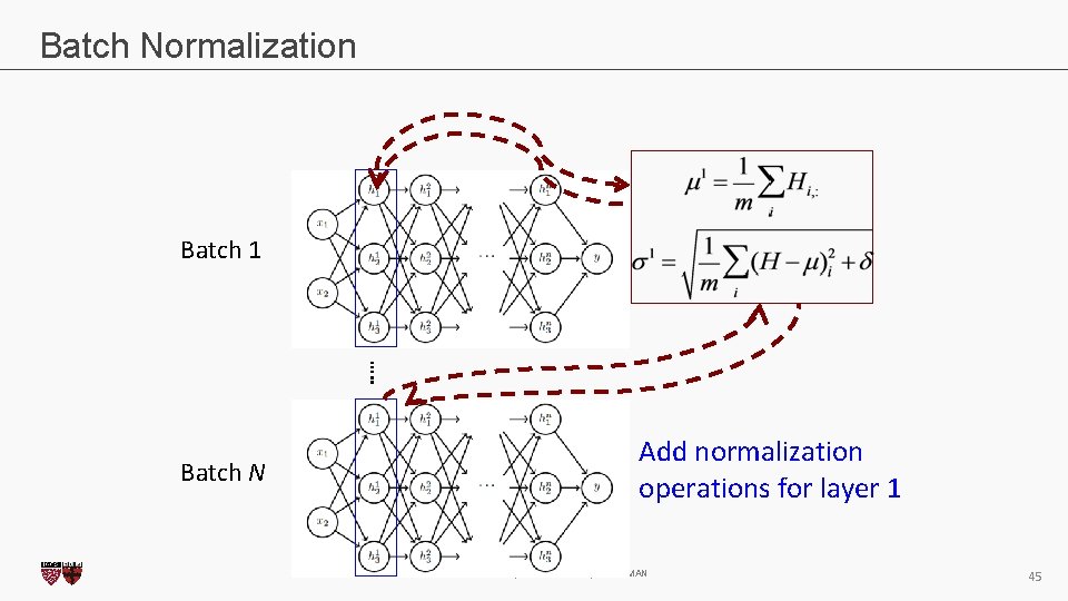
Batch Normalization Batch 1 …. . Batch N Add normalization operations for layer 1 CS 109 B, PROTOPAPAS, GLICKMAN 45

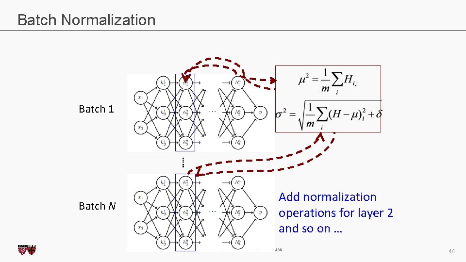
Batch Normalization Batch 1 …. . Batch N Add normalization operations for layer 2 and so on … CS 109 B, PROTOPAPAS, GLICKMAN 46

Batch Normalization Differentiate the joint loss for N mini-batches Back-propagate through the norm operations Test time: – Model needs to be evaluated on a single example – Replace μ and σ with running averages collected during training CS 109 B, PROTOPAPAS, GLICKMAN 47