Lecture 6 Analysis of Categorical and Ordinal Data

Lecture 6 Analysis of Categorical and Ordinal Data: Binomial and Logistic Regression

Analysis of Binary Data l Binomial Regression - l Used when the individual “trial” is not the unit of study, but rather when there are replicates of a set of trials (i. e. seedlings in a quadrat) » In the past, folks often analyzed this type of dataset by converting the response variable to a percentage, and then doing regression on the percentages (after doing ugly transformations…) Model predicts the underlying Binomial probability that would produce the observed number of successes given a number of trials Logistic Regression - Used when the individual Bernoulli trial is the unit of study (i. e. did the seedling die…) Model predicts the probability of “success” of a given trial

Steps in a likelihood analysis for binomial regression In R: 1. Specify the “scientific model” that predicts the probability of “success” as a function of a set of independent variables… -- Note that your scientific model should predict expected values bounded by 0 and 1 (since the predicted value is a probability) 2. Define the likelihood function (using dbinom) binom_log_lh_function <- function(successes, trials, p) { dbinom(x=successes, size=trials, prob = p, log = TRUE) } 3. Set up optimization to find the parameters of the scientific model that maximize likelihood across the dataset

Logistic Regression Example: analysis of windthrow data l Traditionally: Summarize variation in degree and type of damage, across species and tree sizes, from the storm, as a whole. . . l A likelihood alternative: Use the spatial variation in storm intensity that occurs within a given storm to estimate parameters of functions that describe susceptibility to windthrow, as a function of variation in storm severity and individual tree attributes. . .

Types of Response Variables (with examples from analysis of windthrow data) l BINARY: Only two possible outcomes (yes, no; lived, died; etc. ) - This is termed a “Bernoulli trial” l CATEGORICAL: Multiple categories (uprooted, snapped, . . . ) l ORDINAL: Ordered categories (degree of damage): none, light, medium, heavy, complete canopy loss {usually estimated visually} l CONTINUOUS: just what the term implies, but rarely used in analyses of wind damage because of the difficulties of quantifying damage accurately. . .

Analysis of Binary Data: Traditional Logistic Regression Consider a sample space consisting of two outcomes (A, B) where the probability that event A occurs is p Definition: Logit = log of an odds ratio (i. e log[p/(1 -p)]) Benefits of logits • A logit is a continuous variable • Ranges from negative when p < 0. 5 to positive when p > 0. 5 Standard logistic regression involves fitting a linear function to the logit:

What if your terms are multiplicative? Example: Assume that the probability of windthrow is a joint (multiplicative) function of (1) Storm severity, and (2) Tree size In addition, assume that the effect of DBH is nonlinear. . A model that incorporates these can be written as:

A little more detail. . l l Pisj is the probability of windthrow of the jth individual of species s in plot i DBHisj is the DBH of that individual as, bs, and cs are species-specific, estimated parameters, and Si is the estimated storm severity in plot i - NOTE: storm severity is an arbitrary index, and was allowed to range from 0 -1 NOTE: you can think of this as a hierarchical model, with trees nested in plots, and S is the plot term But don’t you have to measure storm severity (not estimate it)?

Likelihood Function for Logistic Regression It couldn’t be any easier. . . (since the scientific model is already expressed as a probabilistic equation): . loglikelihood <- function(pred, observed) { ifelse(observed == 1, log(pred), log(1 -pred)) }

Example: Windthrow in the Adirondacks Highly variable damage due to: • variation within storm • topography • susceptibility of species within a stand Reference: Canham, C. D. , Papaik, M. J. , and Latty, E. F. 2001. Interspecific variation in susceptibility to windthrow as a function of tree size and storm severity for northern temperate tree species. Canadian Journal of Forest Research 31: 1 -10.

The dataset l Study area: 15 x 6 km area perpendicular to the storm path l 43 circular plots: 0. 125 ha (19. 95 m radius) censused in 1996 (20 of the 43 were in oldgrowth forests) l The plots were chosen to span a wide range of apparent damage l All trees > 10 cm DBH censused l Tallied as windthrown if uprooted or if stem was < 45 o from the ground

Critical data requirements l Variation in storm severity across plots l Variation in DBH and species mixture within plots

The analysis. . . l 7 species comprised 97% of stems – only stems of those 7 species were included in the dataset for analysis l # parameters = 64 (43 plots + 3 parameters for each of 7 species) l Parameters estimated using simulated annealing

Model evaluation The solid line is a 1: 1 relationship Numbers above bars represent the number of observations in the class

Estimating Storm Severity

Results: Big trees. . .

Little trees. . .

New twists l Effects of partial harvesting on risk of windthrow to residual trees l Effects of proximity to edges of clearings on risk of windthrow Research with Dave Coates in cedar-hemlock forests of interior B. C.

Effects of harvest intensity and proximity to edge… Equation (1): basic model – probability of windthrow is a species-specific function of tree size and storm severity: Equation (2) introduces the effect of prior harvest removal to equation (1) by adding basal area removal and assumes the effect is independent and additive Equation (3) assumes the effects of prior harvest interact with tree size: Models 1 a – 3 a: test models where separate c coefficients are estimated for “edge” vs. “non-edge” trees (edge = any tree within 10 m of a forest edge)

Other issues… l Is the risk of windthrow independent of the fate of neighboring trees? (not likely) - Should we examine spatially-explicit models that factor in the “nucleating” process of spread of windthrow gaps? …

Analysis for ORDINAL Response Variables l The categories in this case are ranked (i. e. none, light, heavy damage) l Analysis shifts to cumulative probabilities. . .

The “Parallel Slopes” form of ordinal logistic regression l The Challenge: Since the response categories are ordinal, and the model predicts cumulative probabilities, we need a scientific model that generates predictions that keep the categories in order (i. e. the cumulative probability that a response should be in or less than level k needs to be greater than the predicted cumulative probability for level k-1 l The Parallel Slopes solution: - Just allow the intercept term in the equation for the logit to vary among the k ordinal responses, while the slope stays constant (Note that you only need k-1 intercepts…)

Simple Ordinal Logistic Regression If (i. e. the probability that an observation y will be less than or equal to ordinal level Yk (k = 1. . n-1 levels) , given a vector of X explanatory variables), Then simple ordinal logistic regression fits a model of the form: Remember: The probability that an event will fall into a single class k (rather than the cumulative probability) is simply

In our case. . . where and where aks, cs and bs are species specific parameters (s = 1. . S species), and Si are the estimated storm severities for the i = 1. . N plots. # of parameters: N + (K-1+2)*S, where N = # of plots, K = # of ordinal response levels, and S = # of species

The Likelihood Function Stays the Same The probability that an event will fall into a single class k (rather than the cumulative probability) is simply Again, since the scientific model is already expressed as a probabilistic equation:

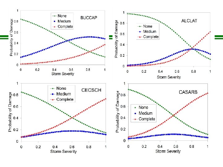
Hurricane Damage in Puerto Rico l Storm damage assessment in the permanent plot at the Luquillo LTER site - l Combined the data into a single analysis: 136 plots, 13 species (including 1 lumped category for “other” species), and 3 damage levels: - l Hurricane Hugo - 1989 Hurricane Georges – 1998 No or light damage Partial damage Complete canopy loss Total # of parameters = 188 (15, 647 trees) Canham, C. D. , J. Thompson, J. K. Zimmerman, and M. Uriarte. 2010. Variation in susceptibility to hurricane damage as a function of storm intensity in Puerto Rican tree species. Biotropica 42: 87 -94.

Parameter Estimation with Simulated Annealing Solving simultaneously for 188 parameters in a dataset containing > 15, 000 trees takes time!

Model Evaluation

Comparison of the two storms. . . Statistics on variation in storm severity from Hurricanes Hugo and Georges