Lecture 6 3 ANOVA 1 way example Analysis

Lecture 6. 3: ANOVA • 1 -way example • Analysis of SS: SSt = SSb + SSw, etc • Use ANOVA formulae to compute F from partial summaries • Contrasts • 2 -way ANOVA • But do HW-4, #K and #I first! 1

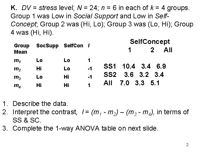
K. DV = stress level; N = 24; n = 6 in each of k = 4 groups. Group 1 was Low in Social Support and Low in Self. Concept; Group 2 was (Hi, Lo); Group 3 was (Lo, Hi); Group 4 was (Hi, Hi). Self. Concept Group Soc. Supp Self. Con l 1 2 All Mean m 1 Lo Lo 1 SS 1 10. 4 3. 4 6. 9 m 2 Hi Lo -1 SS 2 3. 6 3. 2 3. 4 m 3 Lo Hi -1 All 7. 0 3. 3 5. 1 m 4 Hi Hi 1 1. Describe the data. 2. Interpret the contrast, l = (m 1 - m 2) – (m 3 - m 4), in terms of SS & SC. 3. Complete the 1 -way ANOVA table on next slide. 2

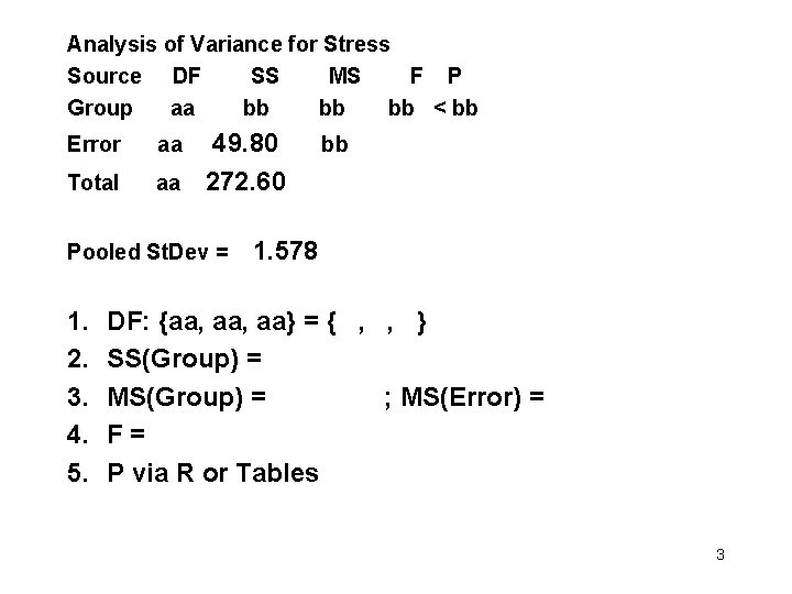
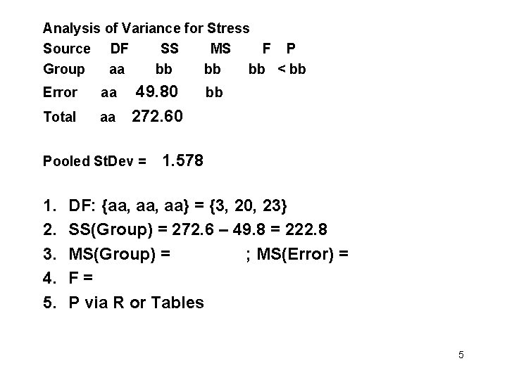
Analysis of Variance for Stress Source DF SS MS F P Group aa bb bb < bb Error aa 49. 80 bb Total aa 272. 60 Pooled St. Dev = 1. 578 1. 2. 3. 4. 5. DF: {aa, aa} = { , , } SS(Group) = MS(Group) = ; MS(Error) = F = P via R or Tables 3

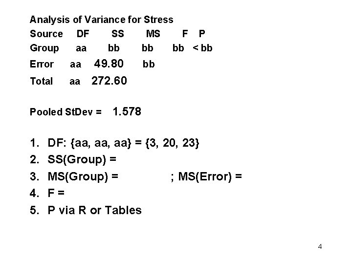
Analysis of Variance for Stress Source DF SS MS F P Group aa bb bb < bb Error aa 49. 80 bb Total aa 272. 60 Pooled St. Dev = 1. 578 1. 2. 3. 4. 5. DF: {aa, aa} = {3, 20, 23} SS(Group) = MS(Group) = ; MS(Error) = F = P via R or Tables 4

Analysis of Variance for Stress Source DF SS MS F P Group aa bb bb < bb Error aa 49. 80 bb Total aa 272. 60 Pooled St. Dev = 1. 578 1. 2. 3. 4. 5. DF: {aa, aa} = {3, 20, 23} SS(Group) = 272. 6 – 49. 8 = 222. 8 MS(Group) = ; MS(Error) = F = P via R or Tables 5

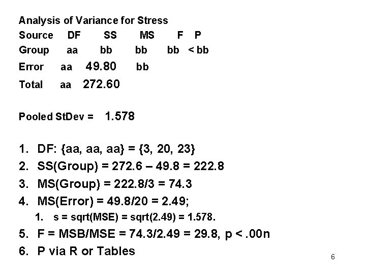
Analysis of Variance for Stress Source DF SS MS F P Group aa bb bb < bb Error aa 49. 80 bb Total aa 272. 60 Pooled St. Dev = 1. 578 1. 2. 3. 4. DF: {aa, aa} = {3, 20, 23} SS(Group) = 272. 6 – 49. 8 = 222. 8 MS(Group) = 222. 8/3 = 74. 3 MS(Error) = 49. 8/20 = 2. 49; 1. s = sqrt(MSE) = sqrt(2. 49) = 1. 578. 5. F = MSB/MSE = 74. 3/2. 49 = 29. 8, p <. 00 n 6. P via R or Tables 6

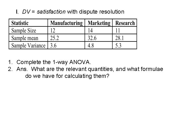
I. DV = satisfaction with dispute resolution 1. Complete the 1 -way ANOVA. 2. Ans. What are the relevant quantities, and what formulae do we have for calculating them?

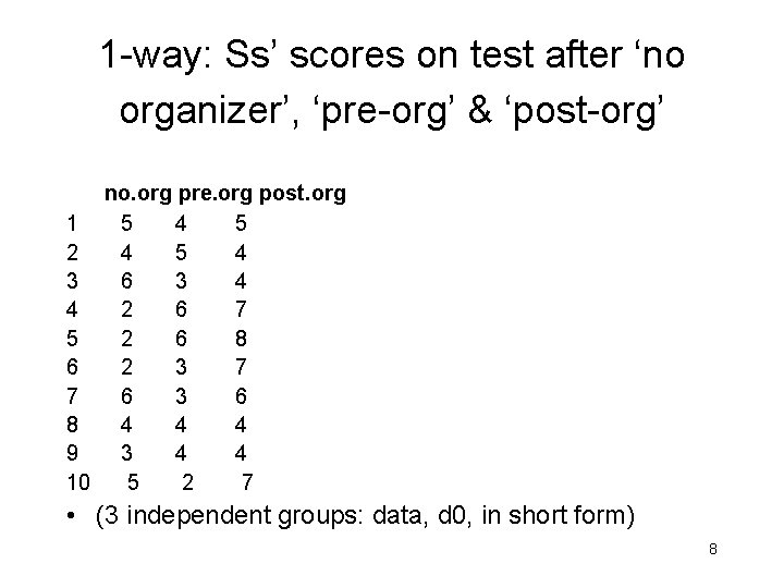
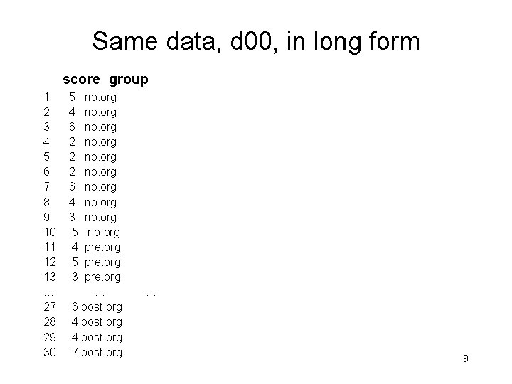
1 -way: Ss’ scores on test after ‘no organizer’, ‘pre-org’ & ‘post-org’ no. org pre. org post. org 1 5 4 5 2 4 5 4 3 6 3 4 4 2 6 7 5 2 6 8 6 2 3 7 7 6 3 6 8 4 4 4 9 3 4 4 10 5 2 7 • (3 independent groups: data, d 0, in short form) 8

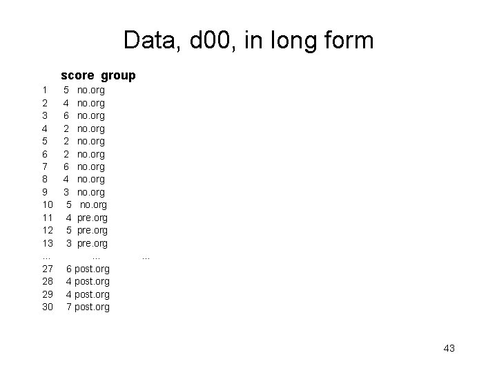
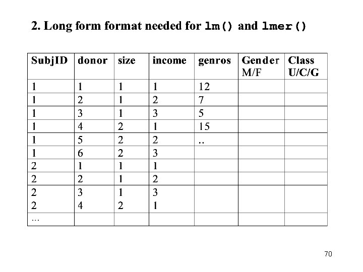
Same data, d 00, in long form score group 1 5 no. org 2 4 no. org 3 6 no. org 4 2 no. org 5 2 no. org 6 2 no. org 7 6 no. org 8 4 no. org 9 3 no. org 10 5 no. org 11 4 pre. org 12 5 pre. org 13 3 pre. org … … 27 6 post. org 28 4 post. org 29 4 post. org 30 7 post. org … 9

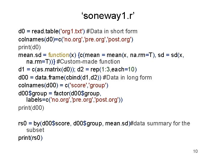
‘soneway 1. r’ d 0 = read. table('org 1. txt') #Data in short form colnames(d 0)=c('no. org', 'pre. org', 'post. org') print(d 0) mean. sd = function(x) {c(mean = mean(x, na. rm=T), sd = sd(x, na. rm=T))} #Custom-made function d 1 = c(as. matrix(d 0)); d 2 = rep(1: 3, each=10) d 00 = data. frame(cbind(d 1, d 2)) #Data in long form colnames(d 00) = c('score', 'group') d 00$group = factor(d 00$group, labels=c('no. org', 'pre. org', 'post. org')) print(d 00) rs 0 = by(d 00$score, d 00$group, mean. sd)#data summary for the subset print(rs 0) 10

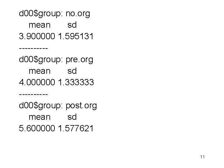
d 00$group: no. org mean sd 3. 900000 1. 595131 -----d 00$group: pre. org mean sd 4. 000000 1. 333333 -----d 00$group: post. org mean sd 5. 600000 1. 577621 11

Week 6: ANOVA • 1 -way example • Analysis of SS: SSt = SSb + SSw, etc • Use ANOVA formulae to compute F from partial summaries • Contrasts • 2 -way ANOVA 12

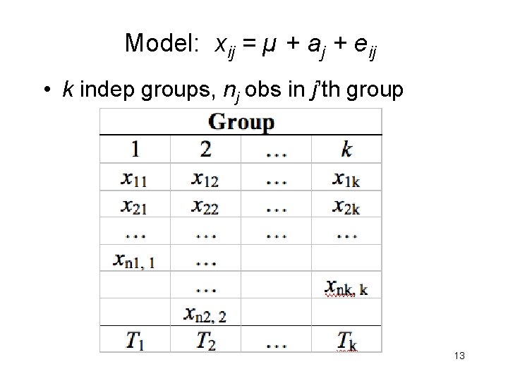
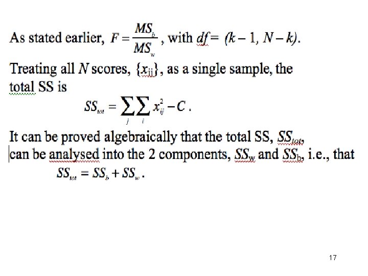
Model: xij = µ + aj + eij • k indep groups, nj obs in j’th group 13

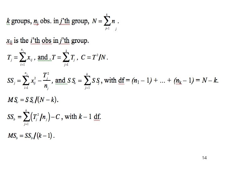
14

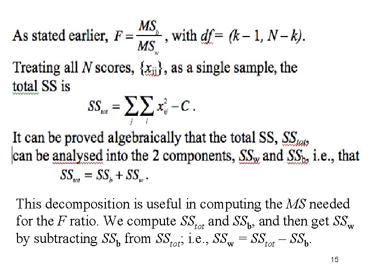
This decomposition is useful in computing the MS needed for the F ratio. We compute SStot and SSb, and then get SSw by subtracting SSb from SStot; i. e. , SSw = SStot – SSb. 15

Use of formulae to compute F from partial summaries • Journal articles sometimes give the means and s. d. s of k groups without F and p-values. Without the raw data you cannot use software to check the statistics; but you can do it ‘by hand’ using the appropriate formulae. • Need to calculate: SSb and SSw; the df of these 2 sums of squares; use the df to compute MSb and MSw; compute the F ratio; and test its significance. 16

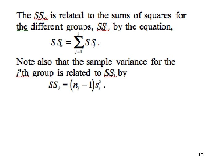
17

18

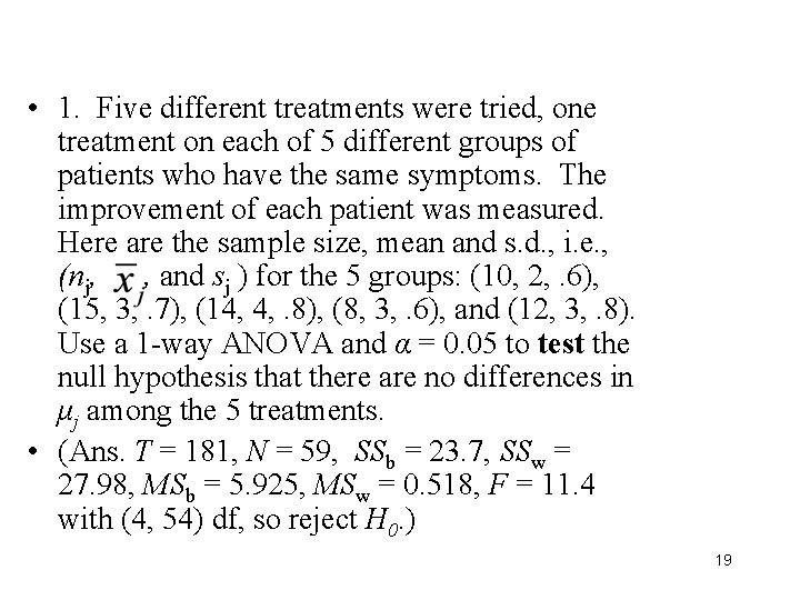
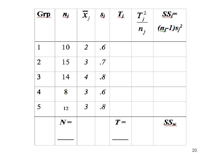
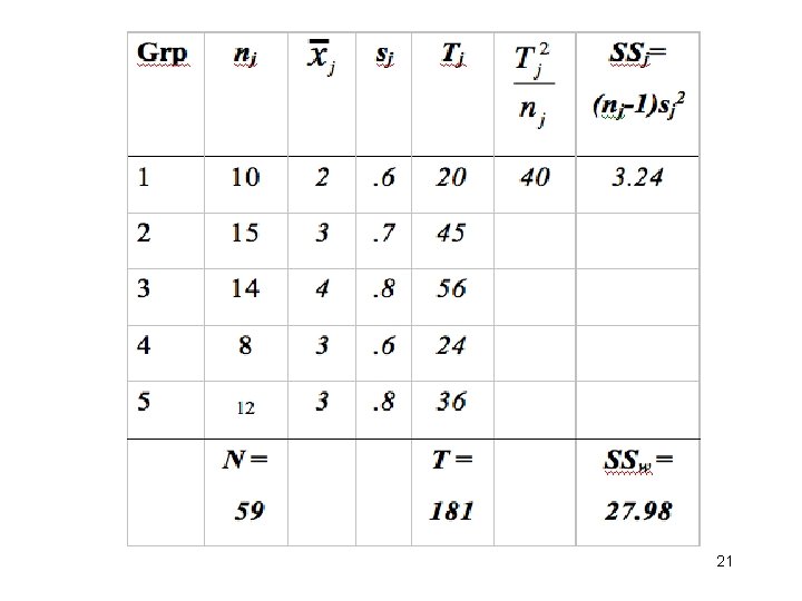
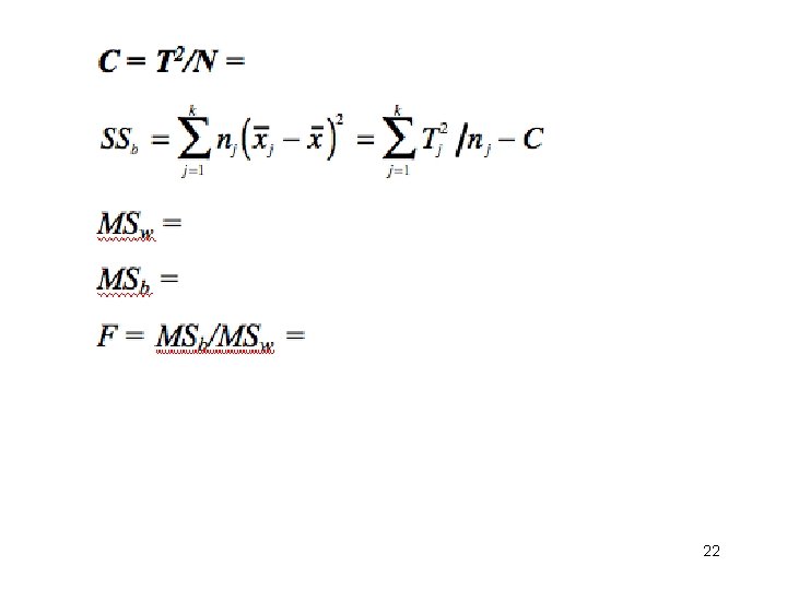
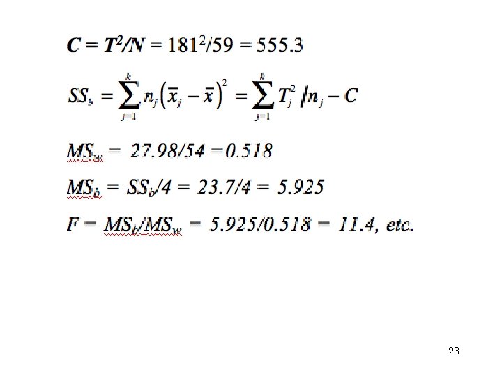
• 1. Five different treatments were tried, one treatment on each of 5 different groups of patients who have the same symptoms. The improvement of each patient was measured. Here are the sample size, mean and s. d. , i. e. , (nj, , and sj ) for the 5 groups: (10, 2, . 6), (15, 3, . 7), (14, 4, . 8), (8, 3, . 6), and (12, 3, . 8). Use a 1 -way ANOVA and α = 0. 05 to test the null hypothesis that there are no differences in μj among the 5 treatments. • (Ans. T = 181, N = 59, SSb = 23. 7, SSw = 27. 98, MSb = 5. 925, MSw = 0. 518, F = 11. 4 with (4, 54) df, so reject H 0. ) 19

20

21

22

23

Week 6: ANOVA • 1 -way example • Analysis of SS: SSt = SSb + SSw, etc • Use ANOVA formulae to compute F from partial summaries • Contrasts • 2 -way ANOVA 24

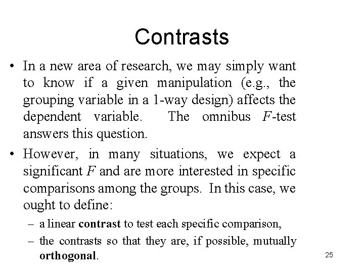
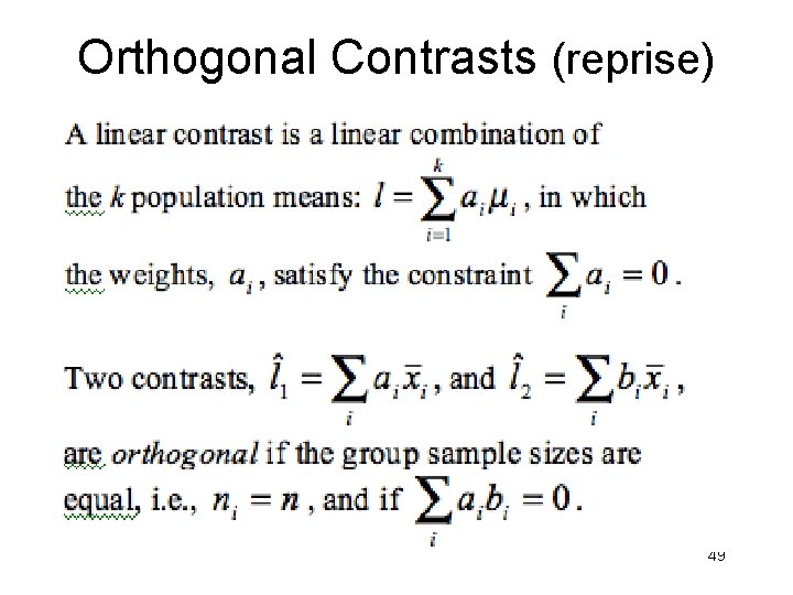
Contrasts • In a new area of research, we may simply want to know if a given manipulation (e. g. , the grouping variable in a 1 -way design) affects the dependent variable. The omnibus F-test answers this question. • However, in many situations, we expect a significant F and are more interested in specific comparisons among the groups. In this case, we ought to define: – a linear contrast to test each specific comparison, – the contrasts so that they are, if possible, mutually orthogonal. 25

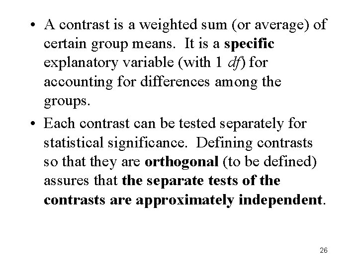
• A contrast is a weighted sum (or average) of certain group means. It is a specific explanatory variable (with 1 df) for accounting for differences among the groups. • Each contrast can be tested separately for statistical significance. Defining contrasts so that they are orthogonal (to be defined) assures that the separate tests of the contrasts are approximately independent. 26

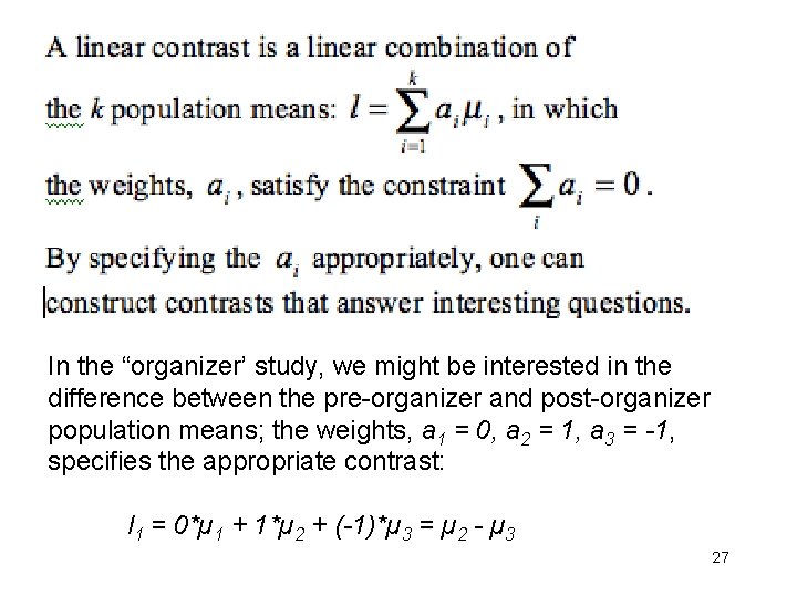
In the “organizer’ study, we might be interested in the difference between the pre-organizer and post-organizer population means; the weights, a 1 = 0, a 2 = 1, a 3 = -1, specifies the appropriate contrast: l 1 = 0*µ 1 + 1*µ 2 + (-1)*µ 3 = µ 2 - µ 3 27

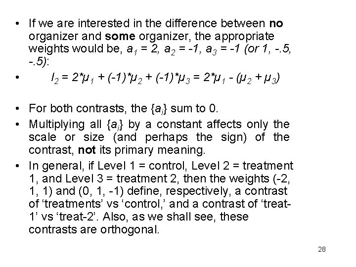
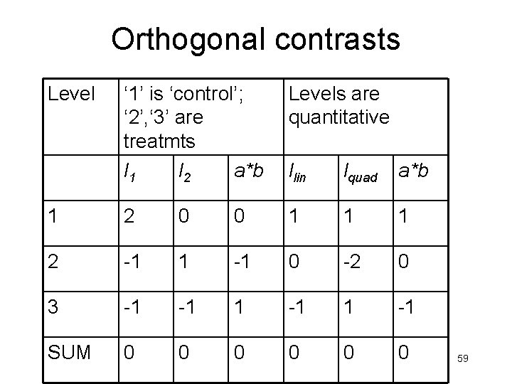
• If we are interested in the difference between no organizer and some organizer, the appropriate weights would be, a 1 = 2, a 2 = -1, a 3 = -1 (or 1, -. 5): • l 2 = 2*µ 1 + (-1)*µ 2 + (-1)*µ 3 = 2*µ 1 - (µ 2 + µ 3) • For both contrasts, the {ai} sum to 0. • Multiplying all {ai} by a constant affects only the scale or size (and perhaps the sign) of the contrast, not its primary meaning. • In general, if Level 1 = control, Level 2 = treatment 1, and Level 3 = treatment 2, then the weights (-2, 1, 1) and (0, 1, -1) define, respectively, a contrast of ‘treatments’ vs ‘control, ’ and a contrast of ‘treat 1’ vs ‘treat-2’. Also, as we shall see, these contrasts are orthogonal. 28

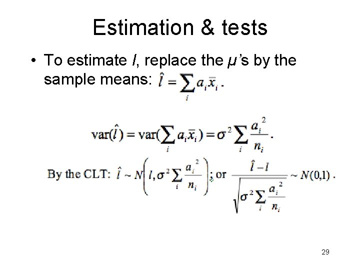
Estimation & tests • To estimate l, replace the µ’s by the sample means: 29

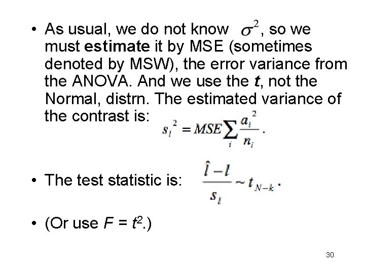
• As usual, we do not know , so we must estimate it by MSE (sometimes denoted by MSW), the error variance from the ANOVA. And we use the t, not the Normal, distrn. The estimated variance of the contrast is: • The test statistic is: • (Or use F = t 2. ) 30

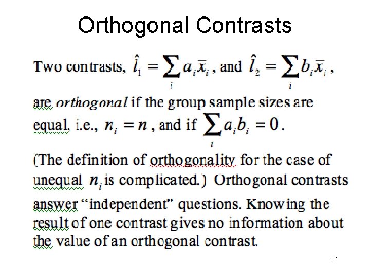
Orthogonal Contrasts 31

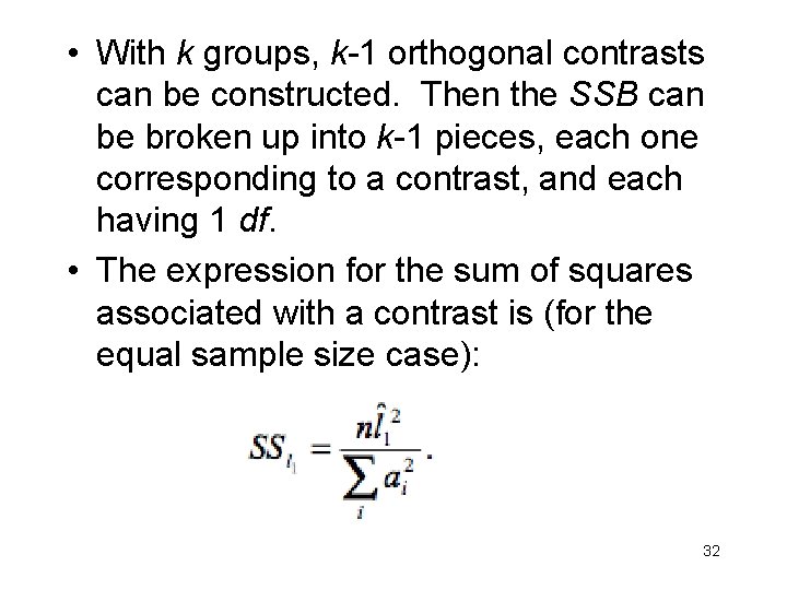
• With k groups, k-1 orthogonal contrasts can be constructed. Then the SSB can be broken up into k-1 pieces, each one corresponding to a contrast, and each having 1 df. • The expression for the sum of squares associated with a contrast is (for the equal sample size case): 32

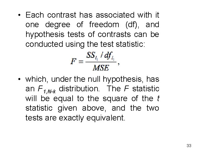
• Each contrast has associated with it one degree of freedom (df), and hypothesis tests of contrasts can be conducted using the test statistic: • which, under the null hypothesis, has an F 1, N-k distribution. The F statistic will be equal to the square of the t statistic given above, and the two tests are exactly equivalent. 33

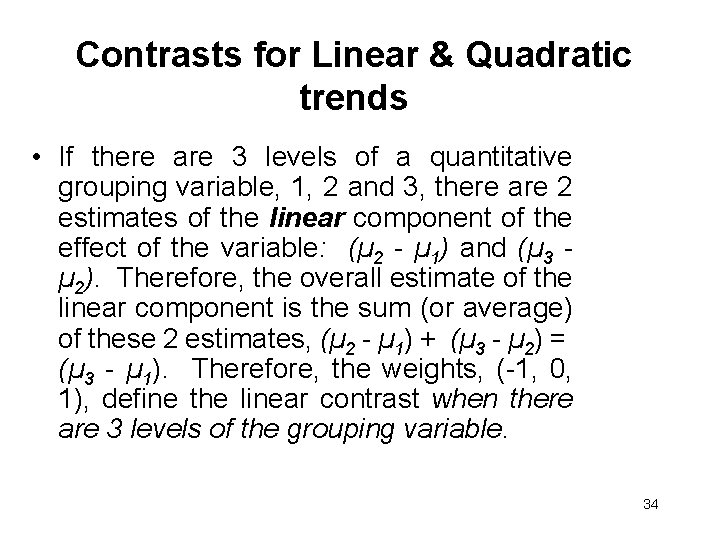
Contrasts for Linear & Quadratic trends • If there are 3 levels of a quantitative grouping variable, 1, 2 and 3, there are 2 estimates of the linear component of the effect of the variable: (µ 2 - µ 1) and (µ 3 µ 2). Therefore, the overall estimate of the linear component is the sum (or average) of these 2 estimates, (µ 2 - µ 1) + (µ 3 - µ 2) = (µ 3 - µ 1). Therefore, the weights, (-1, 0, 1), define the linear contrast when there are 3 levels of the grouping variable. 34

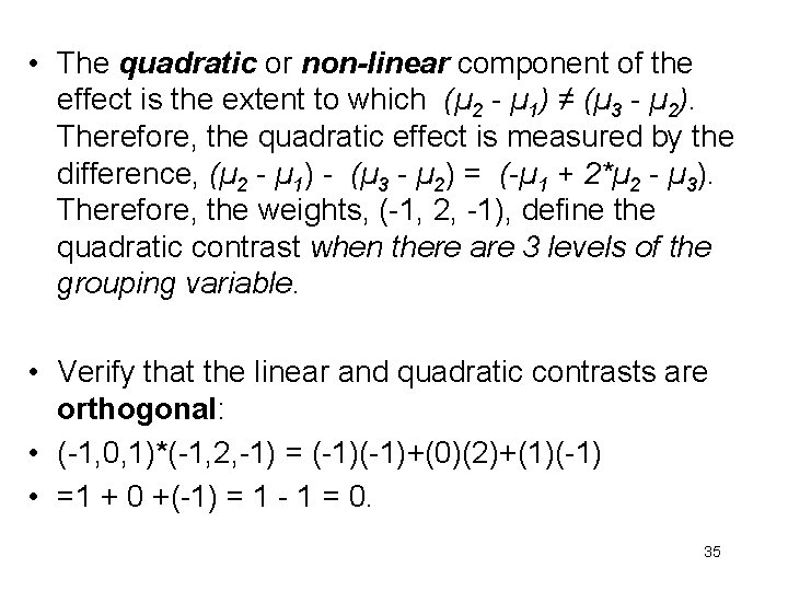
• The quadratic or non-linear component of the effect is the extent to which (µ 2 - µ 1) ≠ (µ 3 - µ 2). Therefore, the quadratic effect is measured by the difference, (µ 2 - µ 1) - (µ 3 - µ 2) = (-µ 1 + 2*µ 2 - µ 3). Therefore, the weights, (-1, 2, -1), define the quadratic contrast when there are 3 levels of the grouping variable. • Verify that the linear and quadratic contrasts are orthogonal: • (-1, 0, 1)*(-1, 2, -1) = (-1)+(0)(2)+(1)(-1) • =1 + 0 +(-1) = 1 - 1 = 0. 35

Lecture 7. 1: ANOVA • Examples of different sets of orthogonal contrasts when k = 4. • What are the predictors or ‘contrasts’ in lm() when contr. treatment(factor, base=1) is used? Dummy Coding. • Algebraic interpretation of coeffs in terms of group means. This depends on the set of ‘contrasts’ used. • Effect Coding and Orthogonal Coding • Multiple comparisons 36

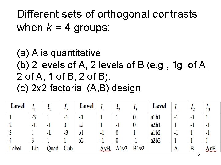
Different sets of orthogonal contrasts when k = 4 groups: (a) A is quantitative (b) 2 levels of A, 2 levels of B (e. g. , 1 g. of A, 2 of A, 1 of B, 2 of B). (c) 2 x 2 factorial (A, B) design 37

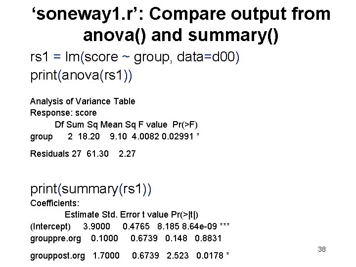
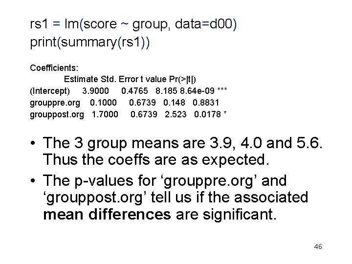
‘soneway 1. r’: Compare output from anova() and summary() rs 1 = lm(score ~ group, data=d 00) print(anova(rs 1)) Analysis of Variance Table Response: score Df Sum Sq Mean Sq F value Pr(>F) group 2 18. 20 9. 10 4. 0082 0. 02991 * Residuals 27 61. 30 2. 27 print(summary(rs 1)) Coefficients: Estimate Std. Error t value Pr(>|t|) (Intercept) 3. 9000 0. 4765 8. 185 8. 64 e-09 *** grouppre. org 0. 1000 0. 6739 0. 148 0. 8831 grouppost. org 1. 7000 0. 6739 2. 523 0. 0178 * 38

• anova(rs 1) gives the familiar omnibus F. • Interestingly, summary(lm()) yields also a set of regression-type coefficients and associated pvalues. What are the ‘predictor’ variables in this regression, and what algebraic interpretation do the coefficients have? • The interpretation of the coeffs depends critically on how the predictors are defined. • The coefficients in the regression will often correspond to the contrasts among group means that we have already discussed. 39

• The predictors will, in general, not look like contrasts among means. However, when the contrasts are orthogonal, the predictors are the same as the contrasts (Benoît). • Note that R calls predictors ‘contrasts’ • What predictors or ‘contrasts’ are used in lm() as the default? Ans: ‘grouppre. org’ and ‘grouppost. org’. • How to (a) specify our own ‘contrasts’, and (b) derive algebraically the interpretation of the coeffs in terms of the group means. 40

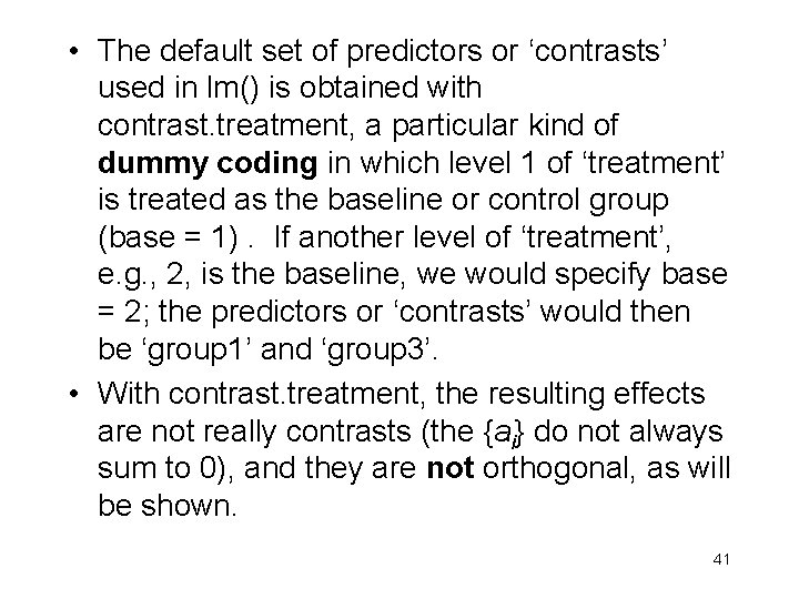
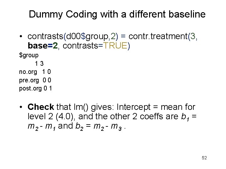
• The default set of predictors or ‘contrasts’ used in lm() is obtained with contrast. treatment, a particular kind of dummy coding in which level 1 of ‘treatment’ is treated as the baseline or control group (base = 1). If another level of ‘treatment’, e. g. , 2, is the baseline, we would specify base = 2; the predictors or ‘contrasts’ would then be ‘group 1’ and ‘group 3’. • With contrast. treatment, the resulting effects are not really contrasts (the {ai} do not always sum to 0), and they are not orthogonal, as will be shown. 41

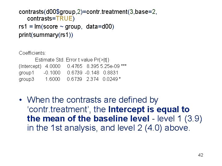
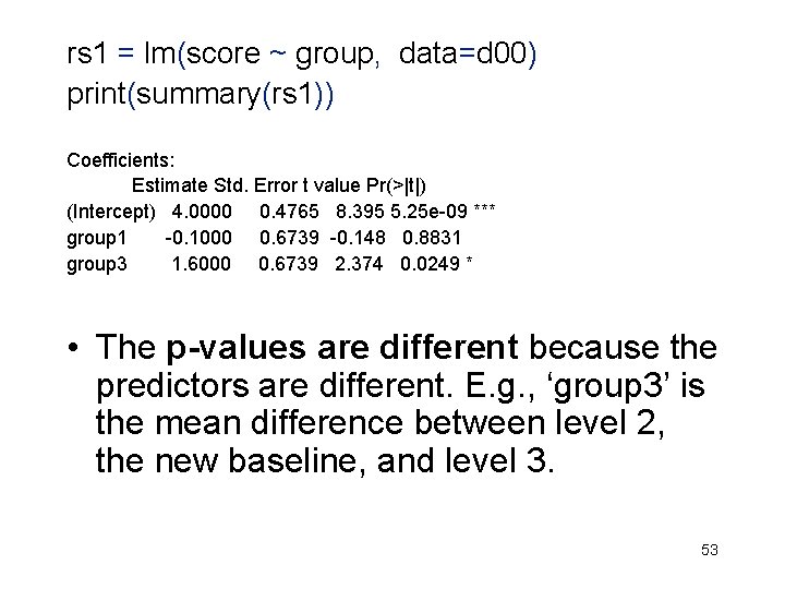
contrasts(d 00$group, 2)=contr. treatment(3, base=2, contrasts=TRUE) rs 1 = lm(score ~ group, data=d 00) print(summary(rs 1)) Coefficients: Estimate Std. Error t value Pr(>|t|) (Intercept) 4. 0000 0. 4765 8. 395 5. 25 e-09 *** group 1 -0. 1000 0. 6739 -0. 148 0. 8831 group 3 1. 6000 0. 6739 2. 374 0. 0249 * • When the contrasts are defined by ‘contr. treatment’, the Intercept is equal to the mean of the baseline level - level 1 (3. 9) in the 1 st analysis, and level 2 (4. 0) above. 42

Data, d 00, in long form score group 1 5 no. org 2 4 no. org 3 6 no. org 4 2 no. org 5 2 no. org 6 2 no. org 7 6 no. org 8 4 no. org 9 3 no. org 10 5 no. org 11 4 pre. org 12 5 pre. org 13 3 pre. org … … 27 6 post. org 28 4 post. org 29 4 post. org 30 7 post. org … 43

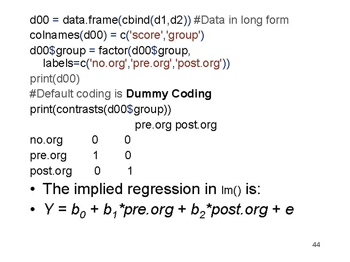
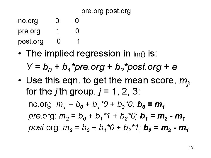
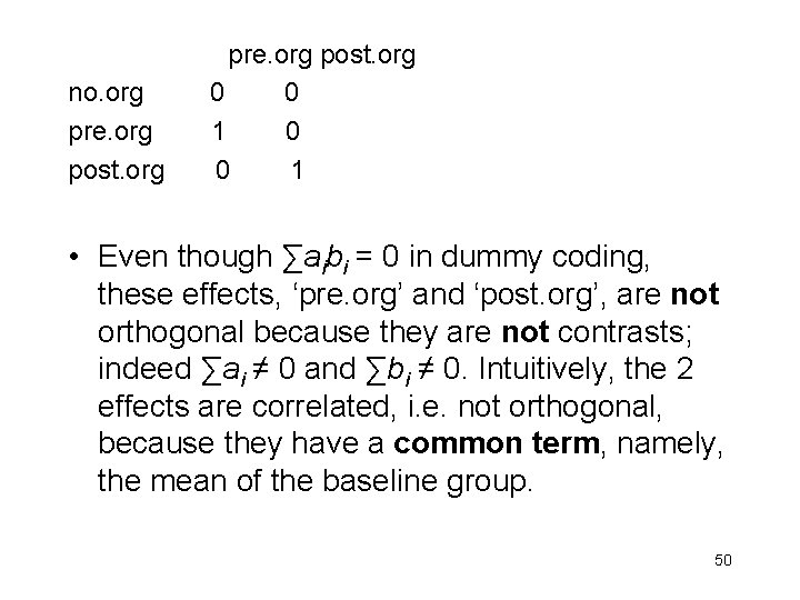
d 00 = data. frame(cbind(d 1, d 2)) #Data in long form colnames(d 00) = c('score', 'group') d 00$group = factor(d 00$group, labels=c('no. org', 'pre. org', 'post. org')) print(d 00) #Default coding is Dummy Coding print(contrasts(d 00$group)) pre. org post. org no. org 0 0 pre. org 1 0 post. org 0 1 • The implied regression in lm() is: • Y = b 0 + b 1*pre. org + b 2*post. org + e 44

pre. org post. org no. org 0 0 pre. org 1 0 post. org 0 1 • The implied regression in lm() is: Y = b 0 + b 1*pre. org + b 2*post. org + e • Use this eqn. to get the mean score, mj, for the j’th group, j = 1, 2, 3: no. org: m 1 = b 0 + b 1*0 + b 2*0; b 0 = m 1 pre. org: m 2 = b 0 + b 1*1 + b 2*0; b 1 = m 2 - m 1 post. org: m 3 = b 0 + b 1*0 + b 2*1; b 2 = m 3 - m 1 45

rs 1 = lm(score ~ group, data=d 00) print(summary(rs 1)) Coefficients: Estimate Std. Error t value Pr(>|t|) (Intercept) 3. 9000 0. 4765 8. 185 8. 64 e-09 *** grouppre. org 0. 1000 0. 6739 0. 148 0. 8831 grouppost. org 1. 7000 0. 6739 2. 523 0. 0178 * • The 3 group means are 3. 9, 4. 0 and 5. 6. Thus the coeffs are as expected. • The p-values for ‘grouppre. org’ and ‘grouppost. org’ tell us if the associated mean differences are significant. 46

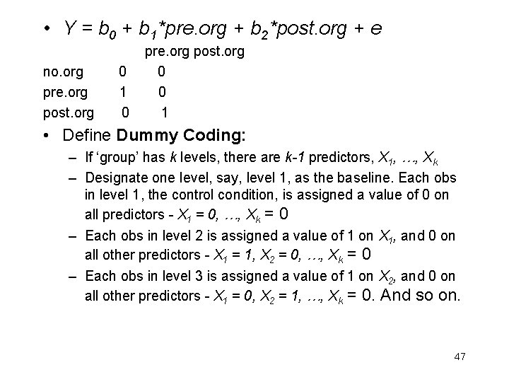
• Y = b 0 + b 1*pre. org + b 2*post. org + e pre. org post. org no. org 0 0 pre. org 1 0 post. org 0 1 • Define Dummy Coding: – If ‘group’ has k levels, there are k-1 predictors, X 1, …, Xk – Designate one level, say, level 1, as the baseline. Each obs in level 1, the control condition, is assigned a value of 0 on all predictors - X 1 = 0, …, Xk = 0 – Each obs in level 2 is assigned a value of 1 on X 1, and 0 on all other predictors - X 1 = 1, X 2 = 0, …, Xk = 0 – Each obs in level 3 is assigned a value of 1 on X 2, and 0 on all other predictors - X 1 = 0, X 2 = 1, …, Xk = 0. And so on. 47

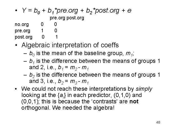
• Y = b 0 + b 1*pre. org + b 2*post. org + e pre. org post. org no. org 0 0 pre. org 1 0 post. org 0 1 • Algebraic interpretation of coeffs – b 0 is the mean of the baseline group, m 1; – b 1 is the difference between the means of groups 1 and 2, i. e. , b 1 = m 2 - m 1 – b 2 is the difference between the means of groups 1 and 3, i. e. , b 2 = m 3 - m 1 • We could not reach these interpretations by simply looking at the {ai} in each predictor, (0, 1, 0) and (0, 0, 1); this is because the ‘contrasts’ are not orthogonal. We needed the algebra! 48

Orthogonal Contrasts (reprise) 49

pre. org post. org no. org 0 0 pre. org 1 0 post. org 0 1 • Even though ∑aibi = 0 in dummy coding, these effects, ‘pre. org’ and ‘post. org’, are not orthogonal because they are not contrasts; indeed ∑ai ≠ 0 and ∑bi ≠ 0. Intuitively, the 2 effects are correlated, i. e. not orthogonal, because they have a common term, namely, the mean of the baseline group. 50

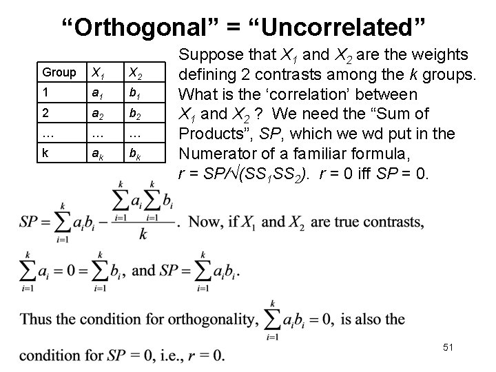
“Orthogonal” = “Uncorrelated” Group X 1 X 2 1 a 1 b 1 2 a 2 b 2 … … … k ak bk Suppose that X 1 and X 2 are the weights defining 2 contrasts among the k groups. What is the ‘correlation’ between X 1 and X 2 ? We need the “Sum of Products”, SP, which we wd put in the Numerator of a familiar formula, r = SP/√(SS 1 SS 2). r = 0 iff SP = 0. 51

Dummy Coding with a different baseline • contrasts(d 00$group, 2) = contr. treatment(3, base=2, contrasts=TRUE) $group 1 3 no. org 1 0 pre. org 0 0 post. org 0 1 • Check that lm() gives: Intercept = mean for level 2 (4. 0), and the other 2 coeffs are b 1 = m 2 - m 1 and b 2 = m 2 - m 3. 52

rs 1 = lm(score ~ group, data=d 00) print(summary(rs 1)) Coefficients: Estimate Std. Error t value Pr(>|t|) (Intercept) 4. 0000 0. 4765 8. 395 5. 25 e-09 *** group 1 -0. 1000 0. 6739 -0. 148 0. 8831 group 3 1. 6000 0. 6739 2. 374 0. 0249 * • The p-values are different because the predictors are different. E. g. , ‘group 3’ is the mean difference between level 2, the new baseline, and level 3. 53

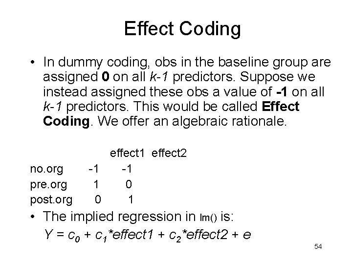
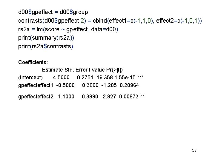
Effect Coding • In dummy coding, obs in the baseline group are assigned 0 on all k-1 predictors. Suppose we instead assigned these obs a value of -1 on all k-1 predictors. This would be called Effect Coding. We offer an algebraic rationale. effect 1 effect 2 no. org -1 pre. org 1 0 post. org 0 1 • The implied regression in lm() is: Y = c 0 + c 1*effect 1 + c 2*effect 2 + e 54

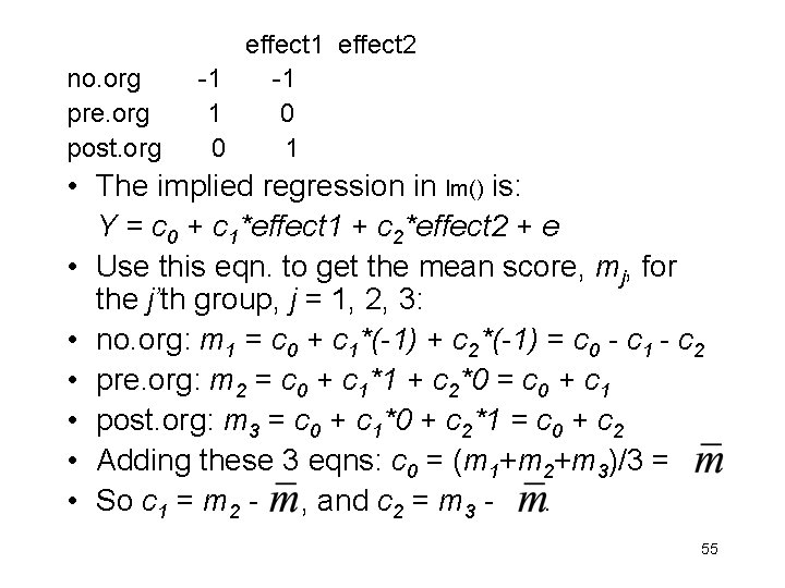
effect 1 effect 2 no. org -1 pre. org 1 0 post. org 0 1 • The implied regression in lm() is: Y = c 0 + c 1*effect 1 + c 2*effect 2 + e • Use this eqn. to get the mean score, mj, for the j’th group, j = 1, 2, 3: • no. org: m 1 = c 0 + c 1*(-1) + c 2*(-1) = c 0 - c 1 - c 2 • pre. org: m 2 = c 0 + c 1*1 + c 2*0 = c 0 + c 1 • post. org: m 3 = c 0 + c 1*0 + c 2*1 = c 0 + c 2 • Adding these 3 eqns: c 0 = (m 1+m 2+m 3)/3 = • So c 1 = m 2 - , and c 2 = m 3 - . 55

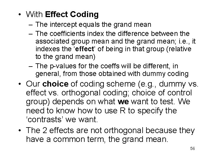
• With Effect Coding – The intercept equals the grand mean – The coefficients index the difference between the associated group mean and the grand mean; i. e. , it indexes the ‘effect’ of being in that group (relative to the grand mean) – The p-values for the coeffs will be different, in general, from those obtained with dummy coding • Our choice of coding scheme (e. g. , dummy vs. effect vs. orthogonal coding; choice of control group) depends on what we want to test. We need to know how to use R to specify the ‘contrasts’ we want. • The 2 effects are not orthogonal because they have a common term, the grand mean. 56

d 00$gpeffect = d 00$group contrasts(d 00$gpeffect, 2) = cbind(effect 1=c(-1, 1, 0), effect 2=c(-1, 0, 1)) rs 2 a = lm(score ~ gpeffect, data=d 00) print(summary(rs 2 a)) print(rs 2 a$contrasts) Coefficients: Estimate Std. Error t value Pr(>|t|) (Intercept) 4. 5000 0. 2751 16. 358 1. 55 e-15 *** gpeffect 1 -0. 5000 0. 3890 -1. 285 0. 20964 gpeffect 2 1. 1000 0. 3890 2. 827 0. 00873 ** 57

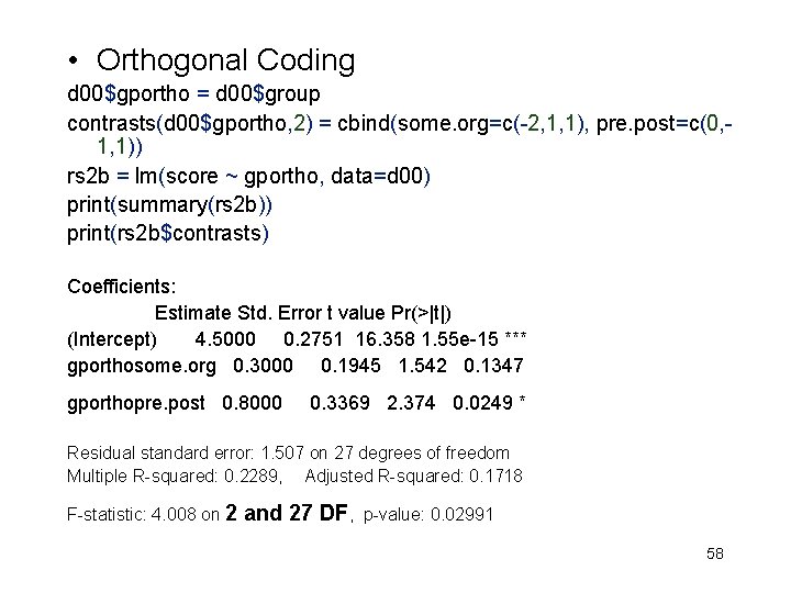
• Orthogonal Coding d 00$gportho = d 00$group contrasts(d 00$gportho, 2) = cbind(some. org=c(-2, 1, 1), pre. post=c(0, 1, 1)) rs 2 b = lm(score ~ gportho, data=d 00) print(summary(rs 2 b)) print(rs 2 b$contrasts) Coefficients: Estimate Std. Error t value Pr(>|t|) (Intercept) 4. 5000 0. 2751 16. 358 1. 55 e-15 *** gporthosome. org 0. 3000 0. 1945 1. 542 0. 1347 gporthopre. post 0. 8000 0. 3369 2. 374 0. 0249 * Residual standard error: 1. 507 on 27 degrees of freedom Multiple R-squared: 0. 2289, Adjusted R-squared: 0. 1718 F-statistic: 4. 008 on 2 and 27 DF, p-value: 0. 02991 58

Orthogonal contrasts Level ‘ 1’ is ‘control’; ‘ 2’, ‘ 3’ are treatmts l 1 l 2 a*b Levels are quantitative llin lquad a*b 1 2 0 0 1 1 1 2 -1 1 -1 0 -2 0 3 -1 -1 SUM 0 0 0 59

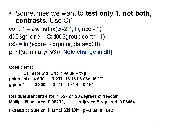
• Sometimes we want to test only 1, not both, contrasts. Use C() contr 1 = as. matrix(c(-2, 1, 1), ncol=1) d 00$grpone = C(d 00$group, contr 1, 1) rs 3 = lm(score ~ grpone, data=d 00) print(summary(rs 3)) [Note change in df!] Coefficients: Estimate Std. Error t value Pr(>|t|) (Intercept) 4. 500 0. 297 15. 151 5. 08 e-15 *** grpone 1 0. 300 0. 210 1. 428 0. 164 Residual standard error: 1. 627 on 28 degrees of freedom Multiple R-squared: 0. 06792, Adjusted R-squared: 0. 03464 F-statistic: 2. 04 on 1 and 28 DF, p-value: 0. 1642 60

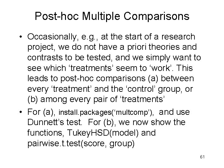
Post-hoc Multiple Comparisons • Occasionally, e. g. , at the start of a research project, we do not have a priori theories and contrasts to be tested, and we simply want to see which ‘treatments’ seem to ‘work’. This leads to post-hoc comparisons (a) between every ‘treatment’ and the ‘control’ group, or (b) among every pair of ‘treatments’ • For (a), install. packages(‘multcomp’), and use Dunnett’s test. For (b), we now show the functions, Tukey. HSD(model) and pairwise. t. test(score, group) 61

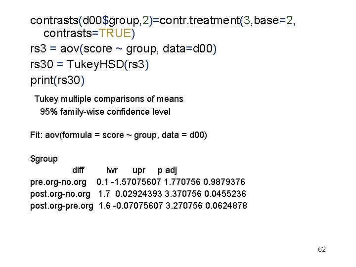
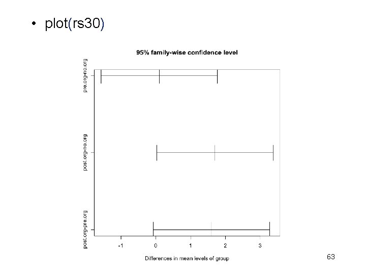
contrasts(d 00$group, 2)=contr. treatment(3, base=2, contrasts=TRUE) rs 3 = aov(score ~ group, data=d 00) rs 30 = Tukey. HSD(rs 3) print(rs 30) Tukey multiple comparisons of means 95% family-wise confidence level Fit: aov(formula = score ~ group, data = d 00) $group diff lwr upr p adj pre. org-no. org 0. 1 -1. 57075607 1. 770756 0. 9879376 post. org-no. org 1. 7 0. 02924393 3. 370756 0. 0455236 post. org-pre. org 1. 6 -0. 07075607 3. 270756 0. 0624878 62

• plot(rs 30) 63

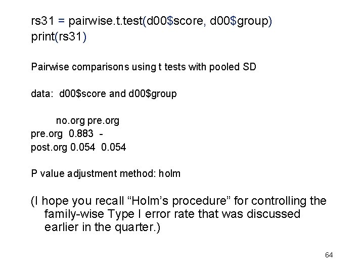
rs 31 = pairwise. t. test(d 00$score, d 00$group) print(rs 31) Pairwise comparisons using t tests with pooled SD data: d 00$score and d 00$group no. org pre. org 0. 883 - post. org 0. 054 P value adjustment method: holm (I hope you recall “Holm’s procedure” for controlling the family-wise Type I error rate that was discussed earlier in the quarter. ) 64

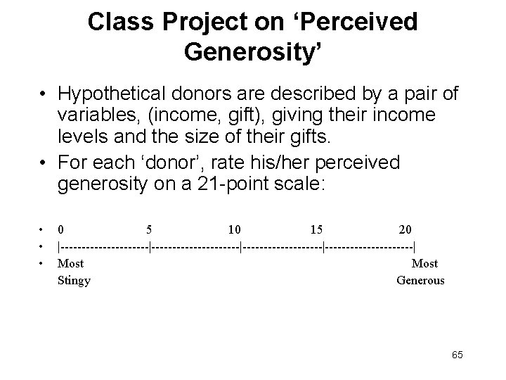
Class Project on ‘Perceived Generosity’ • Hypothetical donors are described by a pair of variables, (income, gift), giving their income levels and the size of their gifts. • For each ‘donor’, rate his/her perceived generosity on a 21 -point scale: • • • 0 5 10 15 20 |---------------------|---------------------| Most Stingy Generous 65

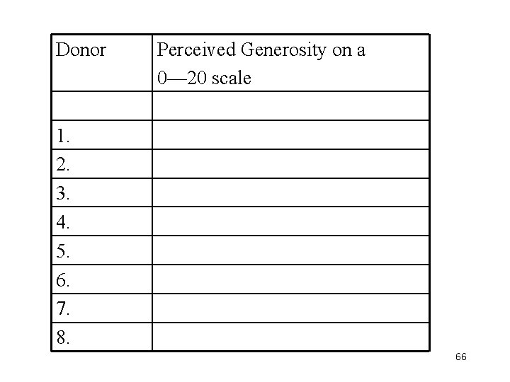
Donor Perceived Generosity on a 0— 20 scale 1. 2. 3. 4. 5. 6. 7. 8. 66

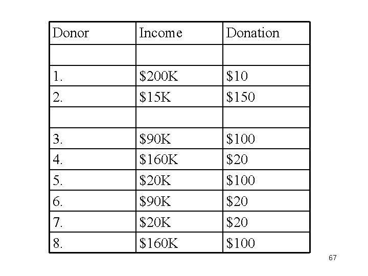
Donor Income Donation 1. 2. $200 K $15 K $10 $150 3. 4. 5. 6. 7. 8. $90 K $160 K $20 K $90 K $20 K $160 K $100 $20 $20 $100 67

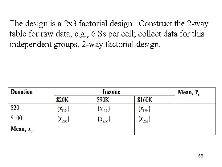
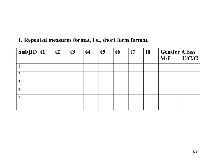
The design is a 2 x 3 factorial design. Construct the 2 -way table for raw data, e. g. , 6 Ss per cell; collect data for this independent groups, 2 -way factorial design. 68

69

70

Aristotle [384 -322 BC], Nicomachean Ethics, IV. i. • … Again, it is those who give whom we call liberal; those who refrain from taking are not praised for Liberality but rather for Justice, and those who take are not praised at all. And of all virtuous people the liberal are perhaps the most beloved, because they are beneficial to others; and they are so in that they give. … 71

• … In crediting people with Liberality their resources must be taken into account; for the liberality of a gift does not depend on its amount, but on the disposition of the giver, and a liberal disposition give according to its substance. It is therefore possible that the smaller give may be the more liberal, if he give from smaller means. … 72

• What next for Meg Whitman, Carly Fiorina? By Ken Mc. Laughlin and Mike Zapler. Mercury News. Posted: 11/03/2010 06: 45: 13 PM PDT • Despite shelling out $141. 5 million of her own, former e. Bay CEO Whitman lost by 12 points to Democrat Jerry Brown, whom Republicans dubbed a career politician and a "retread. " And Fiorina lost to an unpopular Democrat who many political analysts see as too liberal even for California: U. S. Sen. Barbara Boxer. … • Jude Barry, a Democratic strategist in San Jose who ran Westly's campaign, said the two most successful wealthy businessmen turned politicians -- New York Mayor Michael Bloomberg and former Los Angeles Mayor Richard Riordan -- were liked by the voters because they had given generously to charities. • "Voters are mildly impressed with people who make a lot of money and really impressed with people who do good things with it, " Barry said. Despite her estimated wealth of $1. 2 billion, Whitman had no record of being very charitable. 73