Lecture 5 Transfer Functions and Block Diagrams 2

Lecture 5: Transfer Functions and Block Diagrams 2. Transfer function models 3. Intro to block diagrams ME 431, Lecture 5 1. Review differential equation solution process 4. Intro to time response analysis (if time) 1

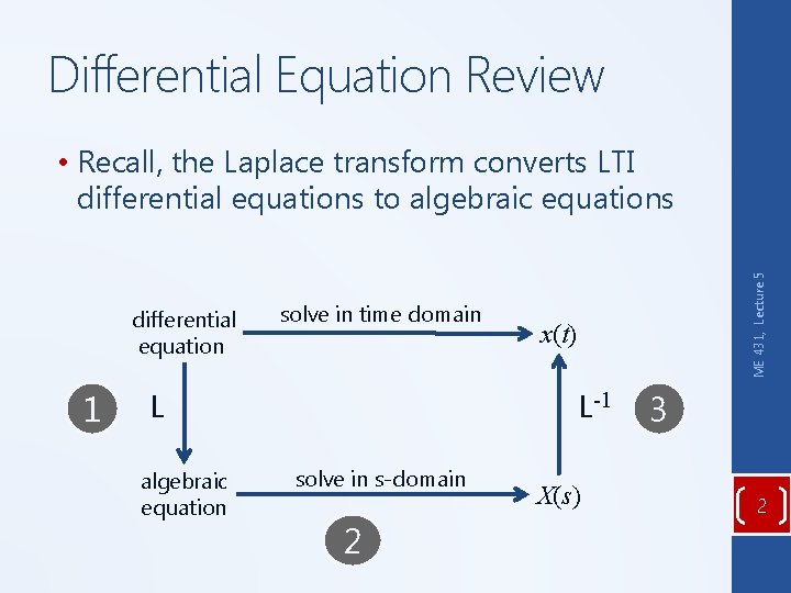
Differential Equation Review differential equation 1 solve in time domain x(t) L-1 L algebraic equation ME 431, Lecture 5 • Recall, the Laplace transform converts LTI differential equations to algebraic equations solve in s-domain 2 X(s) 3 2

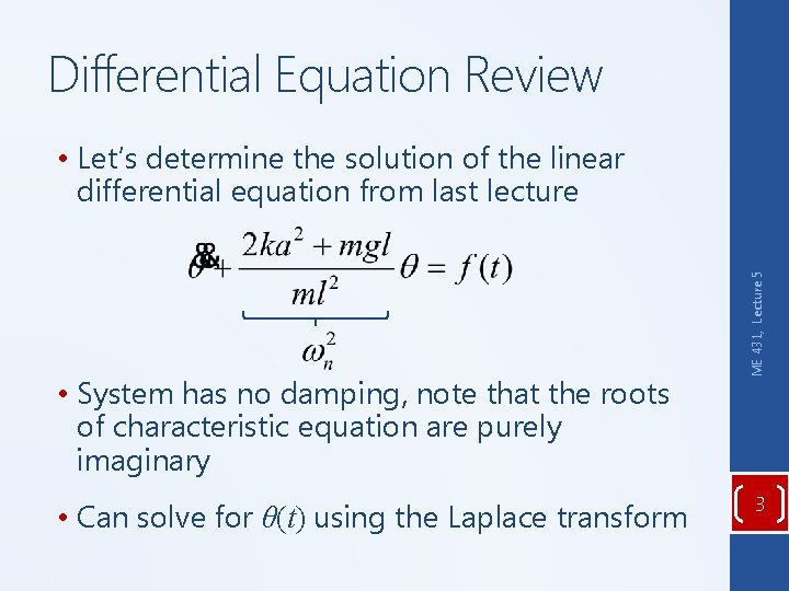
Differential Equation Review • System has no damping, note that the roots of characteristic equation are purely imaginary • Can solve for θ(t) using the Laplace transform ME 431, Lecture 5 • Let’s determine the solution of the linear differential equation from last lecture 3

Example

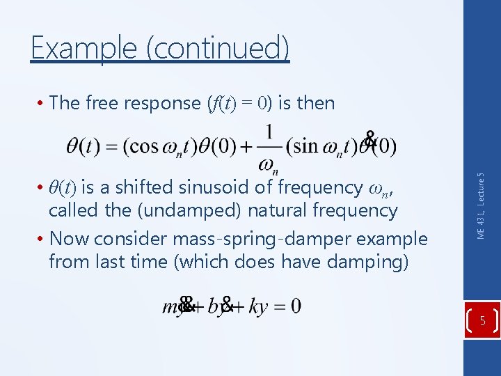
Example (continued) • θ(t) is a shifted sinusoid of frequency ωn, called the (undamped) natural frequency • Now consider mass-spring-damper example from last time (which does have damping) ME 431, Lecture 5 • The free response (f(t) = 0) is then 5

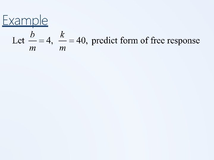
Example

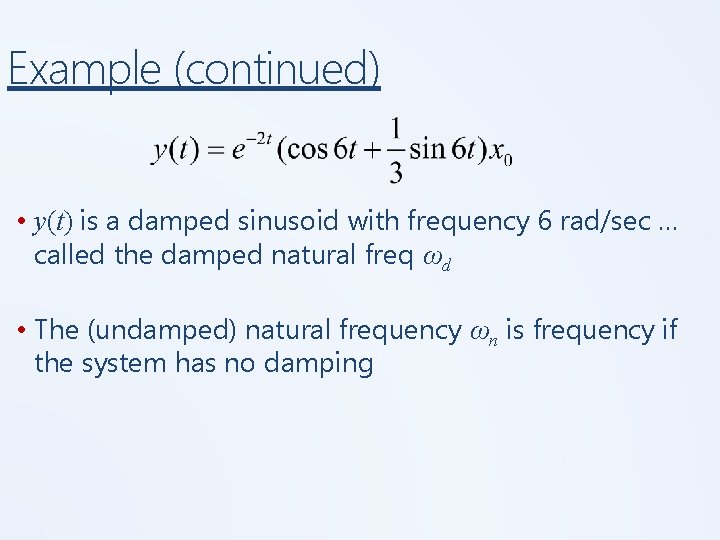
Example (continued) • y(t) is a damped sinusoid with frequency 6 rad/sec … called the damped natural freq ωd • The (undamped) natural frequency ωn is frequency if the system has no damping

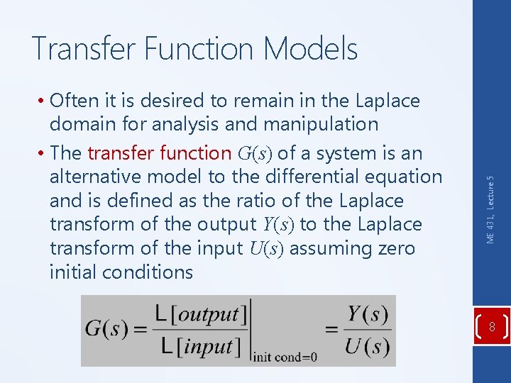
• Often it is desired to remain in the Laplace domain for analysis and manipulation • The transfer function G(s) of a system is an alternative model to the differential equation and is defined as the ratio of the Laplace transform of the output Y(s) to the Laplace transform of the input U(s) assuming zero initial conditions ME 431, Lecture 5 Transfer Function Models 8

• Characterize the input-output relationship of a dynamic system (ignores initial conditions) • Are a property of the system itself, not specific to the particular forcing input (represent natural response) • Have units, but do not provide information concerning the physical structure • Apply only to linear time-invariant (LTI) systems • Make combining systems much easier ME 431, Lecture 5 Transfer Function Models 9

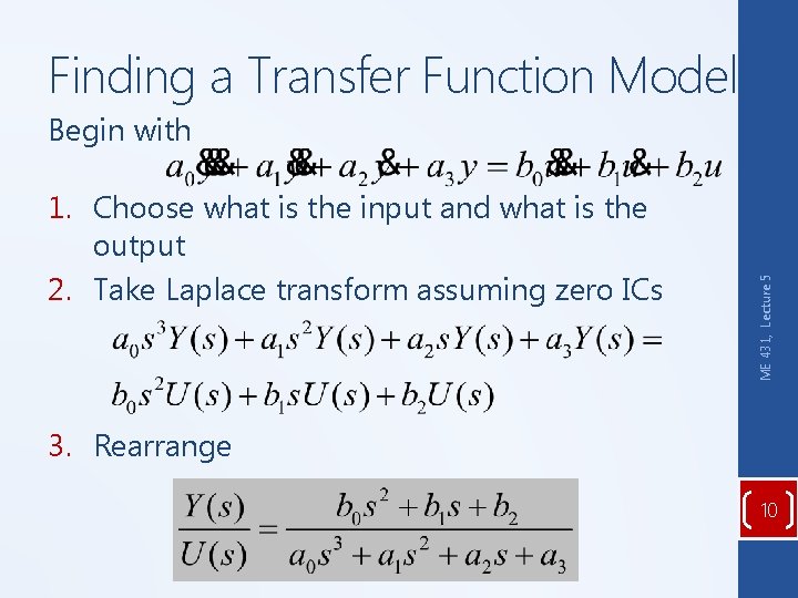
Finding a Transfer Function Model 1. Choose what is the input and what is the output 2. Take Laplace transform assuming zero ICs ME 431, Lecture 5 Begin with 3. Rearrange 10

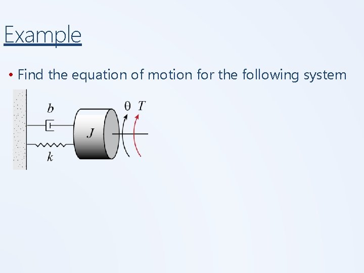
Example • Find the equation of motion for the following system

Example (continued) • Find the transfer function for the previous example where T(t) is the input and θ(t) is the output

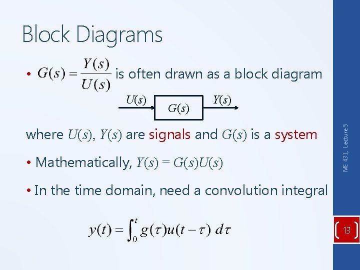
Block Diagrams is often drawn as a block diagram U(s) G(s) Y(s) where U(s), Y(s) are signals and G(s) is a system • Mathematically, Y(s) = G(s)U(s) ME 431, Lecture 5 • • In the time domain, need a convolution integral 13

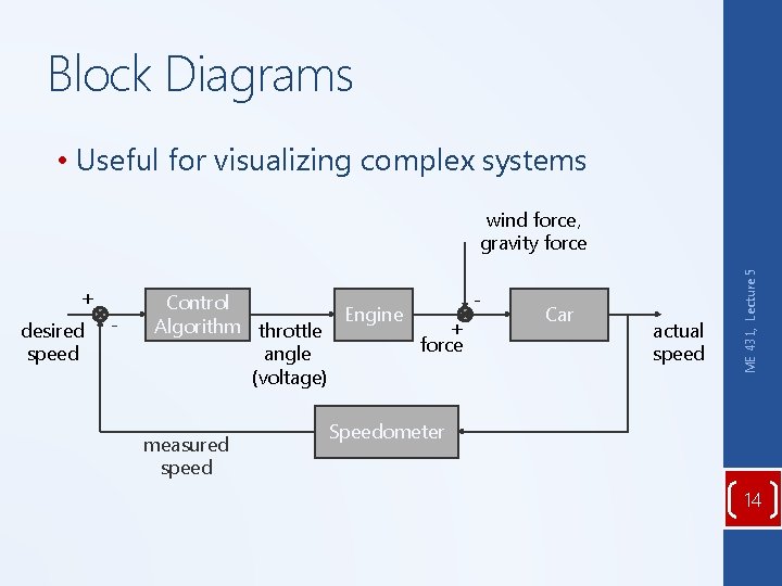
Block Diagrams • Useful for visualizing complex systems + desired speed - Control Engine Algorithm throttle + force angle (voltage) measured speed Car actual speed ME 431, Lecture 5 wind force, gravity force Speedometer 14

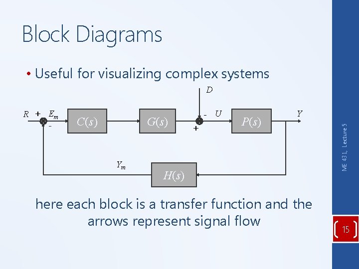
Block Diagrams • Useful for visualizing complex systems D C(s) G(s) Ym - U + P(s) Y H(s) here each block is a transfer function and the arrows represent signal flow ME 431, Lecture 5 R + Em - 15

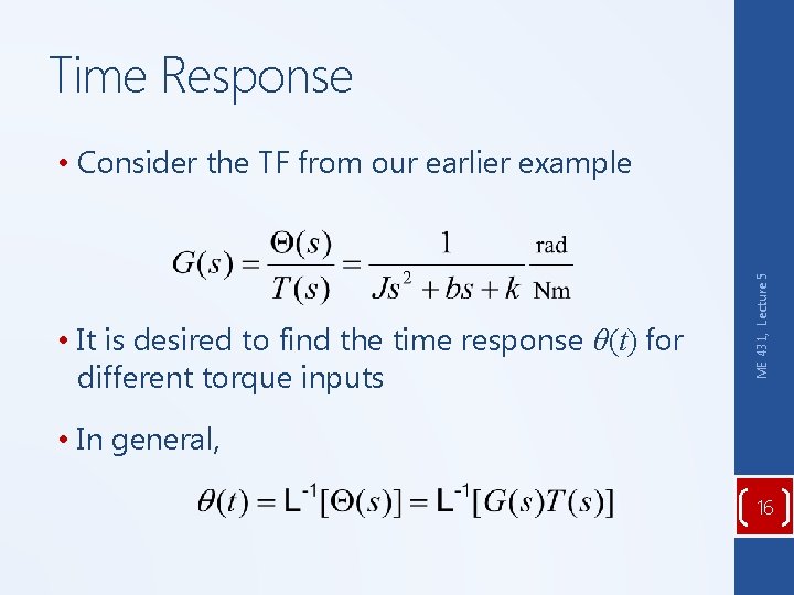
Time Response • It is desired to find the time response θ(t) for different torque inputs ME 431, Lecture 5 • Consider the TF from our earlier example • In general, 16

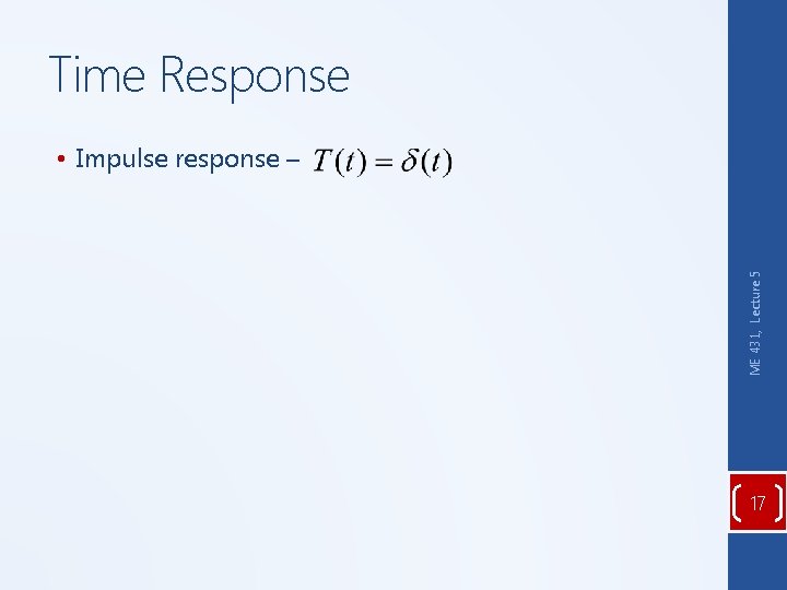
Time Response ME 431, Lecture 5 • Impulse response – 17

ME 431, Lecture 5 MATLAB Notes 18