Lecture 5 Simultaneous Linear Equations Gaussian Elimination 1

Lecture 5 Simultaneous Linear Equations – Gaussian Elimination (1) Dr. Qi Ying

Objectives • Understanding forward elimination and back substitution in Gaussian elimination method • Understanding the concept of singularity and ill-condition

Introduction • Linear equation: each term in each equation contains only one unknown, and each unknown appears to the first power.

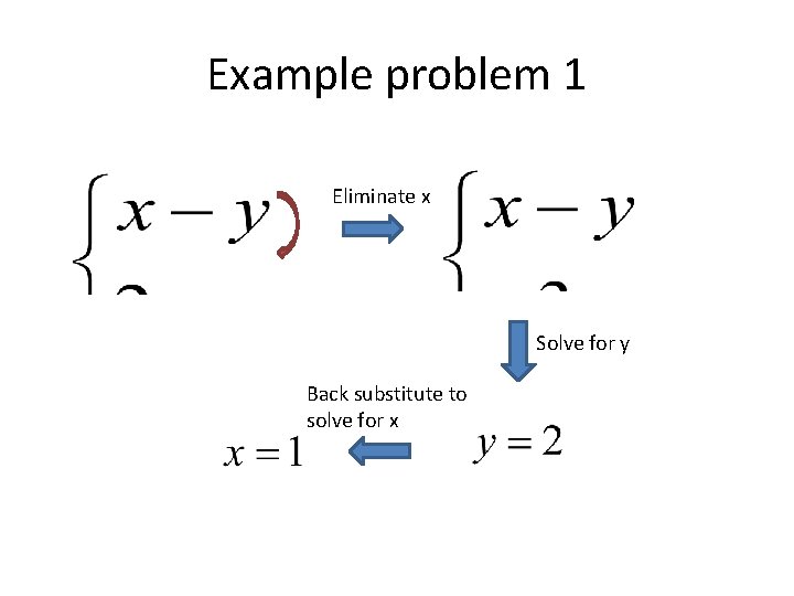
Example problem 1 Eliminate x Solve for y Back substitute to solve for x

Example problem 1 x-y=-1 (x=1, y=2) y 2 x+y=4 X

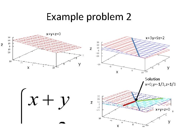
Example problem 2 x+y+z=0 x+3 y+9 z=2 Solution x=0, y=-1/3, z=1/3 x+y+z=0

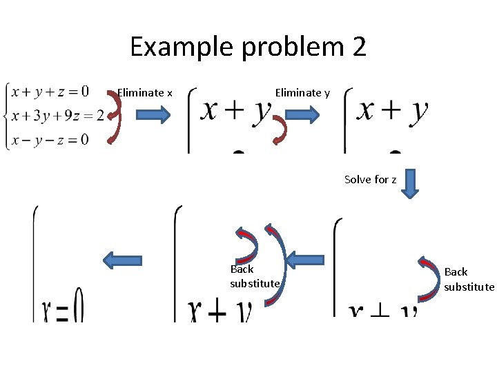
Example problem 2 Eliminate x Eliminate y Solve for z Back substitute

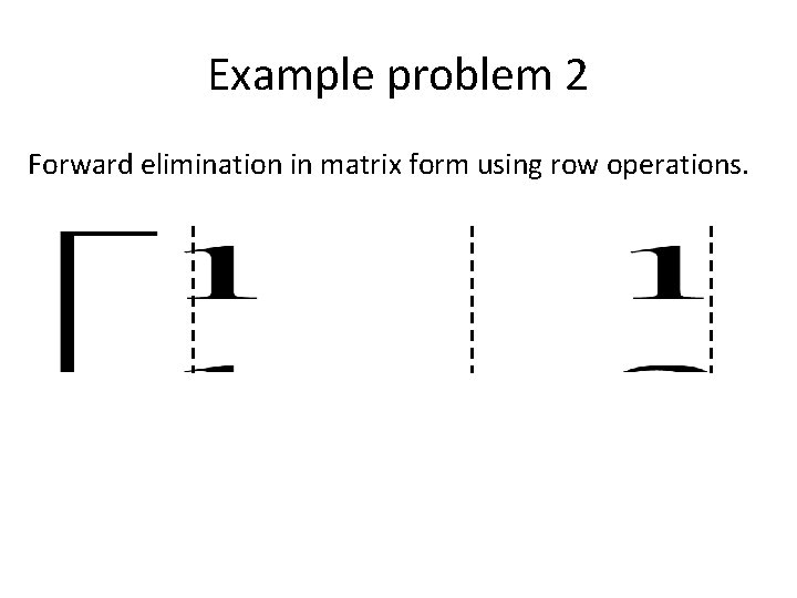
Example problem 2 Forward elimination in matrix form using row operations.

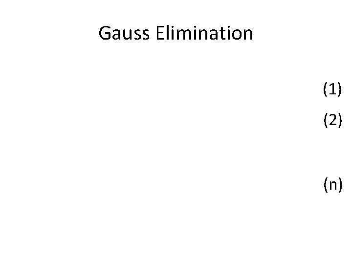
Gauss Elimination (1) (2) (n)

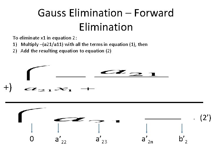
Gauss Elimination – Forward Elimination To eliminate x 1 in equation 2: 1) Multiply –(a 21/a 11) with all the terms in equation (1), then 2) Add the resulting equation to equation (2) +) (2’) 0 a’ 22 a’ 23 a’ 2 n b’ 2

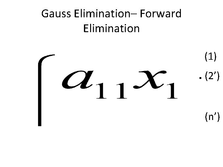
Gauss Elimination– Forward Elimination (1) (2’) (n’)

Gauss Elimination– Forward Elimination

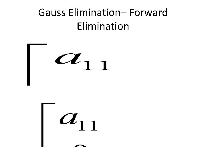
Gauss Elimination– Forward Elimination

Gauss Elimination– Forward Elimination

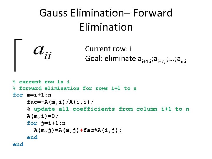
Gauss Elimination– Forward Elimination Current row: i Goal: eliminate ai+1, i; ai+2, i; …; an, i % current row is i % forward elimination for rows i+1 to n for m=i+1: n fac=-A(m, i)/A(i, i); % update all coefficients from column i+1 to n A(m, i)=0; for j=i+1: n A(m, j)=A(m, j)+fac*A(i, j); end

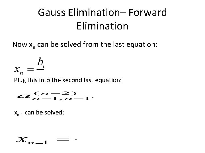
Gauss Elimination– Forward Elimination Now xn can be solved from the last equation: Plug this into the second last equation: xn-1 can be solved:

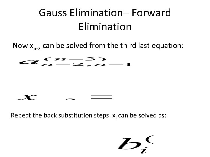
Gauss Elimination– Forward Elimination Now xn-2 can be solved from the third last equation: Repeat the back substitution steps, xi can be solved as:

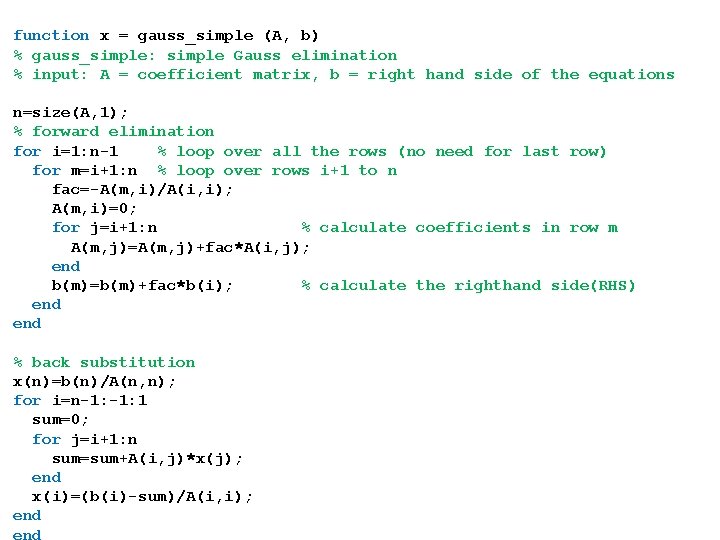
function x = gauss_simple (A, b) % gauss_simple: simple Gauss elimination % input: A = coefficient matrix, b = right hand side of the equations n=size(A, 1); % forward elimination for i=1: n-1 % loop over all the rows (no need for last row) for m=i+1: n % loop over rows i+1 to n fac=-A(m, i)/A(i, i); A(m, i)=0; for j=i+1: n % calculate coefficients in row m A(m, j)=A(m, j)+fac*A(i, j); end b(m)=b(m)+fac*b(i); % calculate the righthand side(RHS) end % back substitution x(n)=b(n)/A(n, n); for i=n-1: 1 sum=0; for j=i+1: n sum=sum+A(i, j)*x(j); end x(i)=(b(i)-sum)/A(i, i); end

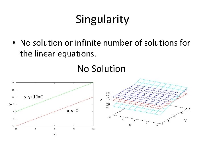
Singularity • No solution or infinite number of solutions for the linear equations. No Solution x-y+10=0 x-y=0

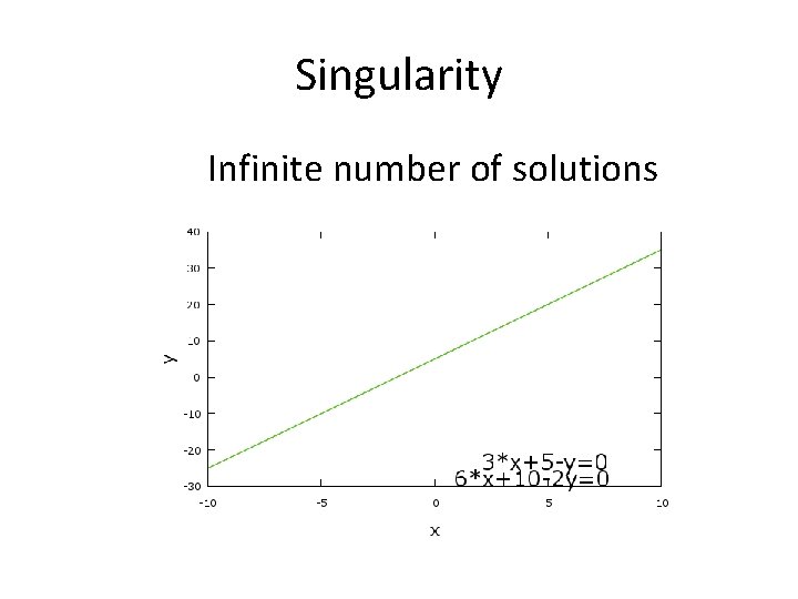
Singularity Infinite number of solutions

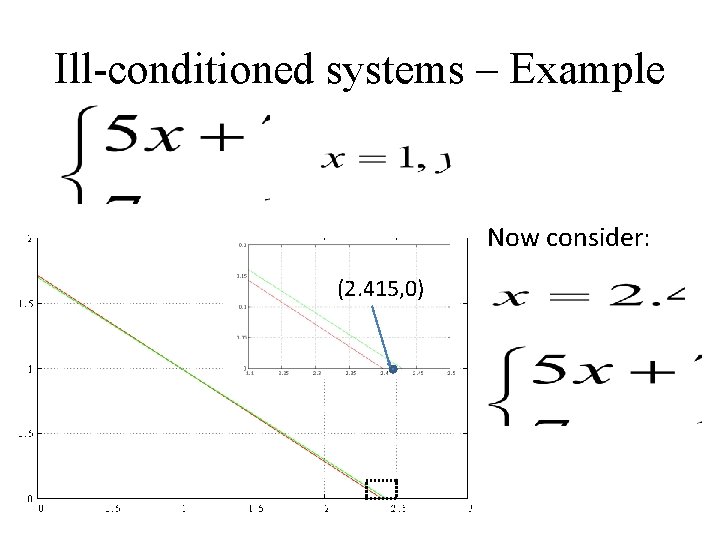
Ill-conditioned systems • A system is either singular or it is not if the operations can be carried out in infinite precision. • In real computer systems, a system can be almost singular, leading to a “solution” that has little reliability.

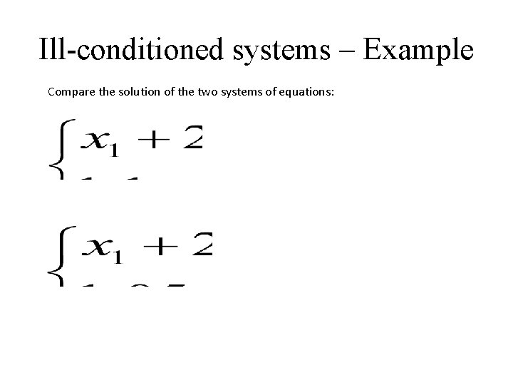
Ill-conditioned systems – Example Compare the solution of the two systems of equations:

Ill-conditioned systems – Example Now consider: (2. 415, 0)

Gauss Elimination – Improvements • Examine the factor used in the forward elimination Fac=-A(m, i)/A(i, i); 1. A(i, i) = 0 -- leads to divide by zero error 2. A(i, i) is close to zero – lead to round-off error. Solution: rearrange the rows so that the ith diagonal element is as large as possible.