Lecture 5 probability model normal distribution binomial distribution

Lecture 5 probability model normal distribution & binomial distribution xiaojinyu@seu. edu. cn

Contents o Normal distribution for continuous data o Binomial distribution for binary categorical data 2

The Normal Distribution The most important distribution in statistics.

Normal distribution o Introduction to normal distribution n n History Parameters and shape standard normal distribution and Z score Area under the curve o Application n Estimate of frequency distribution n Reference interval (range) in health_related field. 4

histroy-Normal Distribution o o o Johann Carl Friedrich Gauss Germany One of the greatest mathematician Applied in physics, astronomy Gaussian distribution (1777~1855) Mark and Stamp in memory of Gauss. 5

The Most Important Distribution o Many real life distributions are approximately normal. such as height, EFV 1, weight, IQ, and so on. o Many other distributions can be almost normalized by appropriate data transformation (e. g. taking the log). When log X has a normal distribution, X is said to have a lognormal distribution. 6

Frequency distributions of heights of adult men. (a) (b) (c) (d) 7

Sample & Population o Histogramo the area of the bars o Cumulative relative frequency o in the sample, the proportion of the boys of age 12 that are lower than a specified height. o o o normal distribution curve The area under the curve The cumulative probability. In the population. Generally speaking, the chance that a boy of aged 12 is lower than a specified height if he grow normally 8

Definition of Normal distribution o X～ N( , 2), X is distributed as normal distribution with mean and variance 2. o The probability density function (PDF) f (x) for a normal distribution is given by (- < X < + ) Where: e = 2. 718285, base of natural logarithm = 3. 1415926536, ratio of the circumference of a circle to the diameter. 9

The shape of a normal distribution f(x) . 4 . 3 . 2 . 1 0 x 10

The normal distributions with the equal variance but different means 3 1 2 11

The normal distributions with the same mean but different variances 2 1 3 12

Properties Of Normal Distribution o & completely determine the characterization of the normal distribution. o Mean, median , mode are equal o The curve is symmetric about mean. o The relationship between and the area under the normal curve provides another main characteristic of the normal distribution. 13

Areas under the Standard Normal Curve o A variable that has a normal distribution with mean 0 and variance 1 is called the standard normal variate and is commonly designated by the letter Z. o N(0, 1) o As with any continuous variable, probability calculations here always concerned with finding the probability that the variable assumes any value in an interval between two specific points a and b. 14

Cumulative distribution Function ( o the area under the curve) from -∞ to x, cumulative Probability S(- , )=1 o Example: What is the probability of obtaining a z value of 0. 5 or less? o We have 15

Area under standard normal distribution (Z) Z -3. 0 -2. 5 -2. 0 -1. 9 -1. 6 -1. 0 -0. 5 0 0. 0013 0. 0062 0. 0228 0. 0287 0. 0548 0. 1587 0. 3085 0. 5000 -0. 02 0. 0013 0. 0059 0. 0217 0. 0274 0. 0526 0. 1539 0. 3015 0. 4920 -0. 04 0. 0012 0. 0055 0. 0207 0. 0262 0. 0505 0. 1492 0. 2946 0. 4840 -0. 06 0. 0011 0. 0052 0. 0197 0. 0250 0. 0485 0. 1446 0. 2877 0. 4761 -0. 08 0. 0010 0. 0049 0. 0188 0. 0239 0. 0465 0. 1401 0. 2810 0. 4681 Z 0 Z is the standard score, that is the units of standard deviation. 16

Figure Standard normal curve and some important divisions. • P(-1 < z < 1)=0. 6826 • P(-2 < z < 2)=0. 9545 • P(-3 < z < 3)=0. 9974 17

Find probability in Excel o Using an electronic table, find the area under the standard normal density to the left of 2. 824. o We use the excel 2007 function NORMSDIST evaluated at 2. 824 [NORMSDIST(2. 824)]with the result as follows: 18

EXAMPLE o What is the probability of obtaining a z value between 1. 0 and 1. 58? o We have 19

CUMULATIVE PROBABILITY FOR X~N(μ, σ2) o Z=(X-μ)/σ -3 -2 - X= μ+Zσ + +2 +3 x 20

Areas under the Normal Curve S(- , )=1 +1 +3 )=0. 6587 +2 )=0. 9987 )=0. 9772 S(- , )=0. 5 -3 )=0. 1587 -2 -1 )=0. 0013 )=0. 0228 21 -3 -2 - -4 -3 -2 -1 0 + +2 +3 1 2 3 4 x Z

Area Under Normal Curve S(- , -3 )=0. 0013 S( -3 , -2 )=0. 0115 S(- , -2 )=0. 0228 S( -2 , -1 )=0. 1359 S(- , -1 )=0. 1587 S( -1 , )=0. 3413 S(- , -0 )=0. 5 -3 -2 - -3 - -2 + +2 -2 -1 0 1 2 + +3 +2 +3 3 22

Area Under Normal Curve 95% 2. 5% -3 -2 +1. 96 -1. 96 -1 0 1 2 3 23

Area Under Normal Curve 90% 5% 5% -3 -2 +1. 64 -1. 64 -1 0 1 2 3 24

Area Under Normal Curve 99% 0. 5% -2. 58 -3 -2 +2. 58 -1 0 1 2 3 25

Area Under Normal Curve 95% 2. 5% -3 -2 +1. 96 -1. 96 -1 0 1 2 3 26

95% heights of females will fall in the range between mean -1. 96 SD and mean +1. 96 SD and

Z score, Standard Score o Transform N( , 2) to N(0, 1 z is refer to as Standard Normal score n How many SD’s the observation from the mean? o Transformation of a normal distribution such that the units are in SD’s. (z score, Standard Score) o By the units of SD, we can compare the observations from diff population. A female with height 172 cm a male with height 172 cm 28

Values of variable & area under curve Observation distributed as normal (x) Standard normal score (Z) AUC（ probability） μ-1σ～μ＋1σ -1～＋1 68. 27% μ-1. 96σ～μ＋1. 96σ -1. 96~1. 96 95. 00% μ-2. 58σ～μ＋2. 58σ -2. 58~2. 58 99. 00% o. The area that falls in the interval under the nonstandard normal curve is the same as that under the standard normal curve within the corresponding u-boundaries. 29

The Most Important Distribution o In practice Many real life distributions are approximately normal, such as height, weight, IQ, GB and so on o In theory Many other distributions can be almost normalized by appropriate data transformation (e. g. taking the log); 30

Summarizing o The fundamental probability distribution of statistics. o A very important distribution both in theory and in practice. o The normal distribution has a set of curves. Defined by mean and SD. (infinite) o N(0, 1) is unique. o The areas under normal curve are equal when measured by standard deviation. 31

Applications of Normal distribution Ø Estimate frequency distribution Ø Estimate Reference Range 32

Estimate frequency distribution Example: o IF the distribution of birth weights follows a normal distribution with mean 3150 g, and standard deviation is 350 g。 o To estimate what proportion of infants whose birth weight are less than 2500 g? 33

Solve for the Example: o The standard normal deviate if x=2500: Z=(x-3150)/350=-1. 86 o The probability when Z<-1. 86 under the standard normal distribution : ϕ(-1. 86)=P(z<-1. 86)=0. 0314 o Result: there about 3. 14% infants whose birth weight are less than 2500 g. 34

Estimate Frequency Distribution 0. 0314 2500 3150 35

Using Normal Distribution o For any variables distributed as normal distribution, 95% individuals assume values between μ-1. 96σ～μ＋1. 96σ; o 99% between -2. 58 ～ +2. 58 ; o And so on. 36

Reference Interval( Range) o In health-related fields, a reference range or reference interval usually describes the variations of a measurement or value in healthy individuals. o It is a basis for a physician or other health professional to interpret a set of results for a particular patient. o The standard definition of a reference range (usually referred to if not otherwise specified) basically originates in what is most prevalent in a reference group taken from the population. However, there also optimal health ranges that are those that appear to have the optimal health impact on people.

Reference Interval( Range) o What is ? n A range of values within which majority of measurements from “normal” subjects will lie. n Majority: 90%，95%，99%, etc. 。 o Usage： n Used as the basis for assessing the result of diagnostic tests in clinic. (normal? abnormal? ) o Definitions of “Normal subject”: n Normal Healthy n maybe suffer from other diseases, but do not influence the variable we studied. 38

How to estimate a reference interval? o o o Homogeneity of normal subjects. 100 Measurement errors are controlled One side? Two sides? Majority? 90%, 95%? Is it necessary to estimated RI in subgroups? (considerations of partitioning based on age, sex etc) o Determine the suspect range if necessary 39

Two-side or One-side o Determined by medical professional. n Two-side: o WBC, BP, serum total cholesterol, …… n One-side: o Upper Limit : urine Ld, hair Hg, …Normal as long as lower than o Low Limit: Vital Capacity, IQ, FEV 1 (forced expiratory volume in one second) o Normal as long as great than 40

Overlap distributed of observations for Normal and Abnormal (one-side) Normal Subject False-negative rate False-positive rate Abnormal 41 界值

Overlap distributed of observations for Normal and Abnormal (one-side) Normal Subject False-negative rate False-positive rate Abnormal 42

Overlap distributed of observations for Normal and Abnormal (two-side) False-negative rate False-positive rate Normal Subject Abnormal 43

Normal approximate method o For normally distributed data o A 95% reference interval n Two-side: n One-side: For upper limit: For low limit:

Percentile Method o For non-normally distributed data o A 95% reference interval n Two-side: n One-side: P 2. 5 ~ P 97. 5 For upper limit: For low limit: <P 95 >P 5 45

Example o Hb (hemoglobin) for 360 normal male. n The mean is 13. 45 g/100 ml; n The standard deviation is 0. 71 g/100 ml; n Hb is normally distributed. o Estimate the 95% reference range and the 90% reference range. 46

Example (cont. ) o Two side o The 95% reference range is 12. 06～ 14. 84 (g/100 ml) 47

Example (cont. ) o Two side The 90% reference range is 12. 29～ 14. 61 (g/100 ml) The 95% reference range is 12. 06～ 14. 84 (g/100 ml) 48

Two methods for reference intervals. Method two-side One-side Low Upper Normal Percentile P 2. 5～P 97. 5 >P 5 <P 95 49

Central Limit Theorem o As a sample size increased, the means of samples drawn from a population of and distribution will approach the normal distribution. This theorem is known as the central limit theorem (CLT). o That is Sampling distributions o Probability and the central limit theorem 50

Sampling distribution o A sampling distribution is the probability distribution of a sample statistic that is formed when samples of size n are repeatedly taken from a population. o The sampling distribution of sample means 51

Binomial Distribution Probability Model for discrete data

Review o binary qualitative data o rate-incidence /proportion-prevalence 53

Tossing coin o What’s the probability that you flip exactly 3 heads in 5 coin tosses? 54

• P(3 heads & 2 tails) =5 C 3*P(heads)3*P(tails)2 • =10*(0. 5)3(0. 5)2=31. 25% • • ways to arrange 3 heads in 5 trials • 5 C 3 Outcome Probability THHHT (1/2)3 * (1/2)2 HHHTT (1/2)3 * (1/2)2 TTHHH (1/2)3 * (1/2)2 HTTHH (1/2)3 * (1/2)2 HHTTH (1/2)3 * (1/2)2 HTHHT (1/2)3 * (1/2)2 THTHH (1/2)3 * (1/2)2 HTHTH (1/2)3 * (1/2)2 HHTHT (1/2)3 * (1/2)2 THHTH (1/2)3 * (1/2)2 = 5!/3!2! = 10 10 arrangements • The probability of each unique outcome (note: they are all equal) (1/2)3 *(1/2)2 • Factorial review: n! = n(n-1)(n-2)… 55

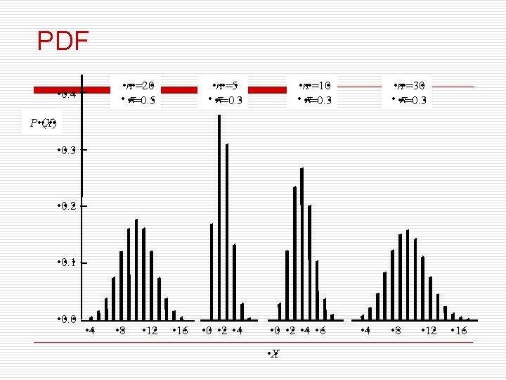
Binomial distribution function: X= the number of heads tossed in 5 coin tosses • p(x) • 0 • 1 • 2 • 3 • 4 • 5 • x • number of heads 56

Example for side effect of drug o if a certain drug is known to cause a side effect 10% of the time and if five patients are given this drug, what is the probability that four or more experience the side effect? o Let S denote a side-effect outcome and N an outcome without side effects. 57

Table 58

Solution to example o The probability of obtaining an outcome with four S’s and one N is o The probability of obtaining all five S’s is o the probability of the compound event that ‘‘four or more have side effects is 59

probability density function(PDF) o The model is concerned with the total number of successes in n trials as a o random variable, denoted by X. Its probability density function is given by nthe number of combinations of x objects selected from a set of n 60

Assumptions for Binomial Distribution o The experiment consists of n repeated trials satisfying these assumptions: o 1. The n trials are all independent. o 2. The parameter p of one in 2 is the same for each trial. 61

The mean and variance of the binomial distribution nwhen the number of trials n is from moderate to large (n > 25, say), we approximate the binomial distribution by a normal distribution and answer probability questions by first converting to a standard normal score: n where π is the probability of having a positive outcome from a single trial 62

Solution to Example o For π =0. 1 and n =30, we have 63

65

Review – experiment & survey o 2 type of researches_ experimental and observational research o Clinical trial (4 phases) o Statistical consideration in clinical trial o Controlled /Randomization/blindness/ replication (appropriate sample size). o probabilistic sampling techniques 66

Review on idea of probability

Idea of probability o Definitions of probability o o o Classic probability- If a random experiment can result in n possible mutually exclusive and equally likely outcomes and if n. A of these outcomes have an attribute A, then the probability (Pr) of A is written as n. A /n Statistical probability-If an experiment is performed n times and if n. A of these result in the outcome A, then the probability of A occurring is defined as the limiting ratio: P(A)=n. A/n Subjective probability-Probability represents one’s belief regarding the likelihood of an outcome A occurring o Probability of Event = p 0 <= p <= 1 68

Rule for Computing o If A and B have no outcomes in common, they can not occur simultaneously, they are Mutually Exclusive events P(A or B) = P(A) + P(B) o if events A & B are independent then P(A&B) = P(A)*P(B) 69

Conditional Probability o Concern the odds of one event occurring, given that another event has occurred o P(A|B)=Prob of A, given B o if A and B are independent, then P(B|A) = P(A)*P(B)/P(A) P(B|A) = P(B) 70

Percentile calculation

Quartiles o Quartiles divide data into four equal parts n First quartile—Q 1 o 25% of observations are below Q 1 and 75% above Q 1 o Also called the lower quartile n Second quartile—Q 2 o 50% of observations are below Q 2 and 50% above Q 2 o This is also the median n Third quartile—Q 3 o 75% of observations are below Q 3 and 25% above Q 3 o Also called the upper quartile

Calculating percentiles Example The sorted observations are: 2, 5, 9, 12, 14, 15, 18, 24, 60, find the median and P 20. Solution The number of observations n = 9 12 -73

Calculating percentiles The sorted observations are: 4, 9, 10, 12, 14, 20, 24, 61, Find the median and P 20. o (n+1)*20%=1. 8 12 -74

• Calculation of percentile from a grouped frequency table • Example: The frequency distribution for the systolic blood pressure readings (in mm or mercury) of 200 randomly selected college students is shown here. Boundaries Frequency cumulative frequency cumulative percent(%) 89. 5 - 24 24 12 104. 5 - 62 86 43 119. 5 - 72 158 79 134. 5 - 26 184 92 149. 5 - 12 196 95 164. 5 - 4 200 100 n. The class interval that contains the relevant quartile is called the quartile class 75

Calculation of quartiles from a grouped frequency table where: L = the real lower limit of the quartile class (containing Q 1 or Q 3) n = Σf = the total number of observations in the entire data set C = the cumulative frequency in the class immediately before the quartile class f = the frequency of the relevant quartile class i = the length of the real class interval of the relevant quartile class 12 -76

• Calculation of percentile from a grouped frequency table class Frequency (f) cumulative frequency(C) cumulative percent(%) 89. 5 - 24 24 12 104. 5 - 62 86 43 119. 5 - 72 158 79 134. 5 - 26 184 92 149. 5 - 12 196 95 164. 5 - 4 200 100 n. The class interval that contains the relevant quartile is called the quartile class 77

• Calculation of quartiles from a grouped frequency table 78