LECTURE 5 Parabolic PDEs 1 Aim of Lecture

LECTURE 5 Parabolic PDEs 1

Aim of Lecture • So far in previous lectures we have discussed: – Elliptic partial differential equations - Laplace and Poisson’s Equations – Discretisation using Finite Differences – Use of Excel to solve Elliptic PDEs • This week we will discuss – Parabolic PDEs – Solution of Parabolic PDEs using Finite Difference Methods – Explicit and Implicit Methods – Solving Parabolic PDEs using Excel 2

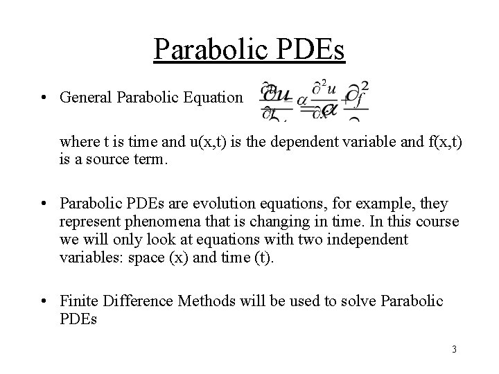
Parabolic PDEs • General Parabolic Equation where t is time and u(x, t) is the dependent variable and f(x, t) is a source term. • Parabolic PDEs are evolution equations, for example, they represent phenomena that is changing in time. In this course we will only look at equations with two independent variables: space (x) and time (t). • Finite Difference Methods will be used to solve Parabolic PDEs 3

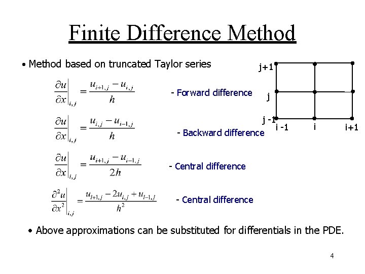
Finite Difference Method • Method based on truncated Taylor series - Forward difference j+1 j j -1 i -1 - Backward difference i i+1 - Central difference • Above approximations can be substituted for differentials in the PDE. 4

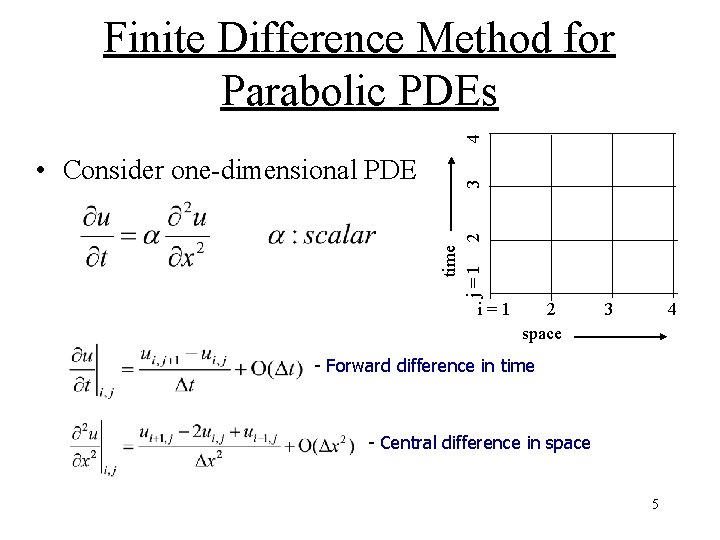
time j=1 2 • Consider one-dimensional PDE 3 4 Finite Difference Method for Parabolic PDEs i=1 2 space 3 4 - Forward difference in time - Central difference in space 5

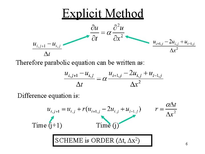
Explicit Method Therefore parabolic equation can be written as: Difference equation is: Time (j+1) Time (j) SCHEME is ORDER ( t, x 2) 6

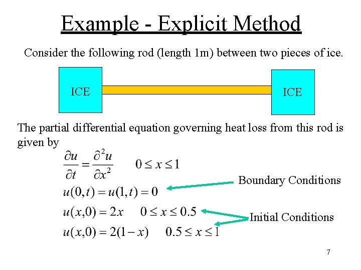
Example - Explicit Method Consider the following rod (length 1 m) between two pieces of ice. ICE The partial differential equation governing heat loss from this rod is given by Boundary Conditions Initial Conditions 7

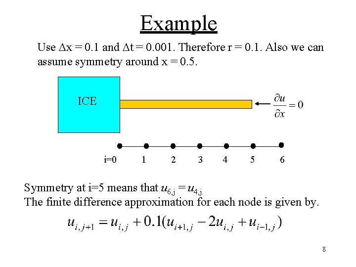
Example Use x = 0. 1 and t = 0. 001. Therefore r = 0. 1. Also we can assume symmetry around x = 0. 5. ICE i=0 1 2 3 4 5 6 Symmetry at i=5 means that u 6, j = u 4, j. The finite difference approximation for each node is given by. 8

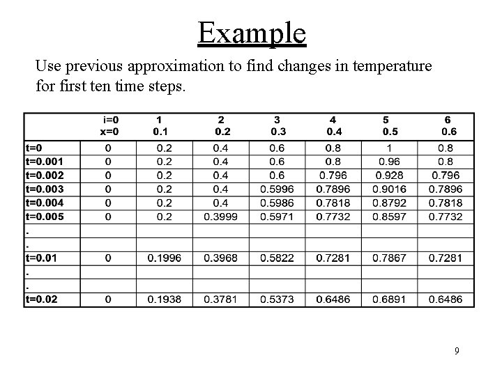
Example Use previous approximation to find changes in temperature for first ten time steps. 9

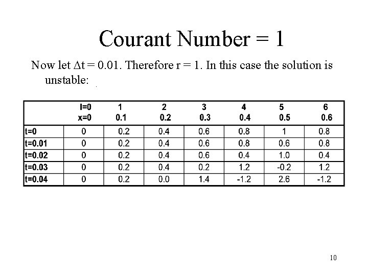
Courant Number = 1 Now let t = 0. 01. Therefore r = 1. In this case the solution is unstable: . 10

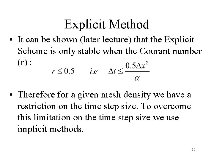
Explicit Method • It can be shown (later lecture) that the Explicit Scheme is only stable when the Courant number (r) : • Therefore for a given mesh density we have a restriction on the time step size. To overcome this limitation on the time step size we use implicit methods. 11

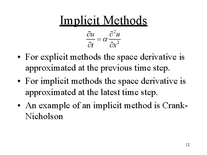
Implicit Methods • For explicit methods the space derivative is approximated at the previous time step. • For implicit methods the space derivative is approximated at the latest time step. • An example of an implicit method is Crank. Nicholson 12

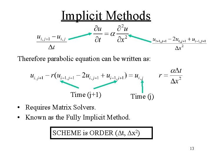
Implicit Methods Therefore parabolic equation can be written as: Time (j+1) Time (j) • Requires Matrix Solvers. • Known as the Fully Implicit Method. SCHEME is ORDER ( t, x 2) 13

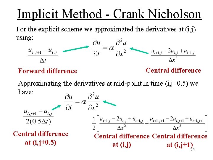
Implicit Method - Crank Nicholson For the explicit scheme we approximated the derivatives at (i, j) using: Forward difference Central difference Approximating the derivatives at mid-point in time (i, j+0. 5) we have: Central difference at (i, j+0. 5) Central difference at (i, j) at (i, j+1) 14

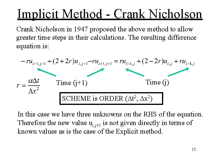
Implicit Method - Crank Nicholson in 1947 proposed the above method to allow greater time steps in their calculations. The resulting difference equation is: Time (j+1) Time (j) SCHEME is ORDER ( t 2, x 2) In this case we have three unknowns on the RHS of the equation. Therefore the new value ui, j+1 is not given directly in terms of known values as is the case of the Explicit method. 15

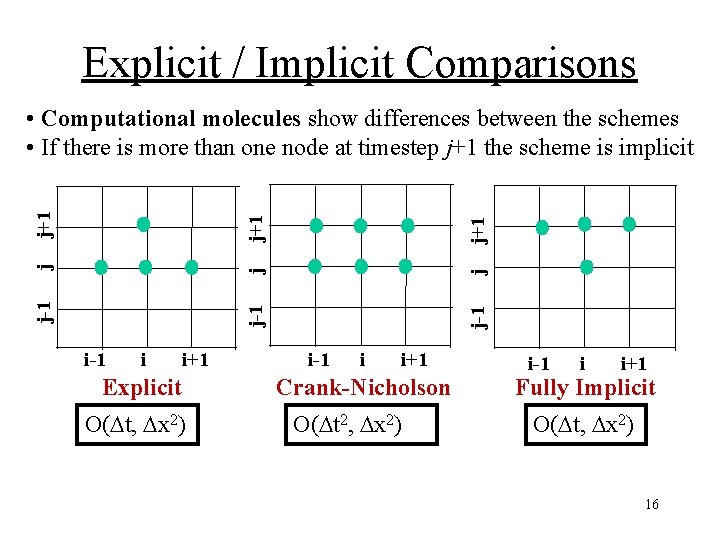
Explicit / Implicit Comparisons i-1 i i+1 Explicit O( t, x 2) j+1 j j-1 j-1 j j j+1 • Computational molecules show differences between the schemes • If there is more than one node at timestep j+1 the scheme is implicit i-1 i i+1 Crank-Nicholson O( t 2, x 2) i-1 i i+1 Fully Implicit O( t, x 2) 16

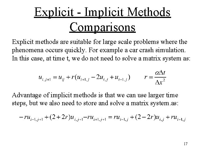
Explicit - Implicit Methods Comparisons Explicit methods are suitable for large scale problems where the phenomena occurs quickly. For example a car crash simulation. In this case, at time t, we do not need to solve a matrix system as: Advantage of implicit methods is that we can use larger time steps, but we also need to store and solve a matrix system. as: 17

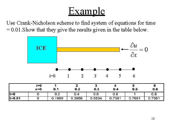
Example Use Crank-Nicholson scheme to find system of equations for time = 0. 01. Show that they give the results given in the table below. ICE i=0 1 2 3 4 5 6 18

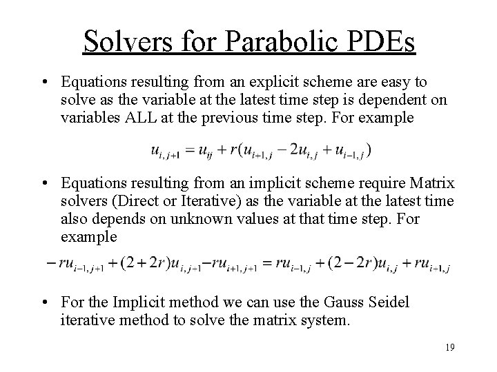
Solvers for Parabolic PDEs • Equations resulting from an explicit scheme are easy to solve as the variable at the latest time step is dependent on variables ALL at the previous time step. For example • Equations resulting from an implicit scheme require Matrix solvers (Direct or Iterative) as the variable at the latest time also depends on unknown values at that time step. For example • For the Implicit method we can use the Gauss Seidel iterative method to solve the matrix system. 19

Excel for Solving Parabolic PDEs using Finite Difference Equations 20

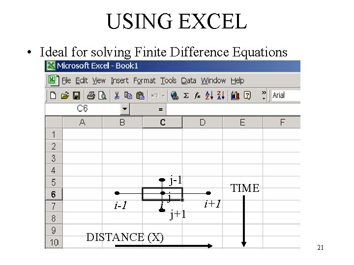
USING EXCEL • Ideal for solving Finite Difference Equations i-1 i j-1 j j+1 TIME i+1 DISTANCE (X) 21

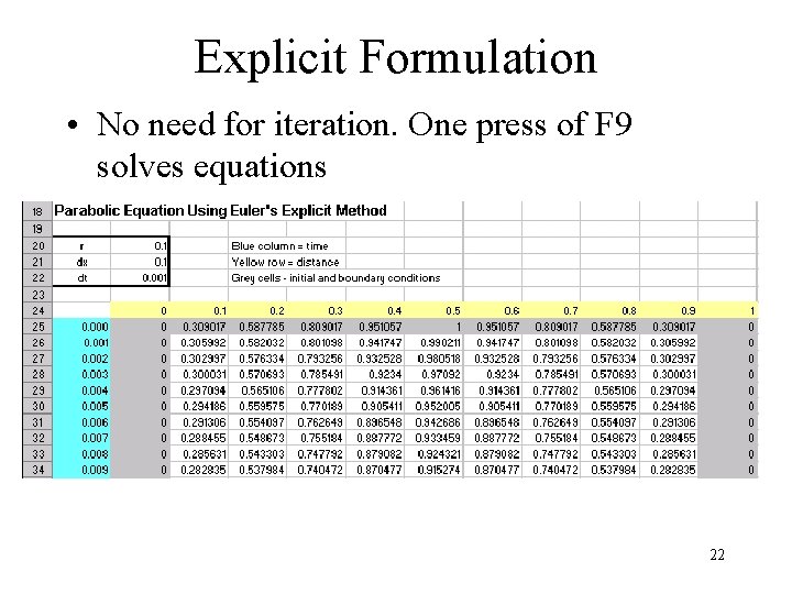
Explicit Formulation • No need for iteration. One press of F 9 solves equations 22

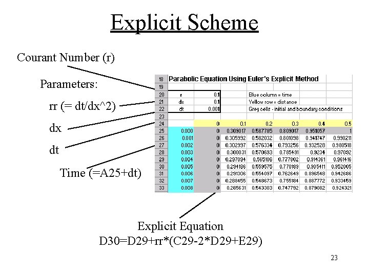
Explicit Scheme Courant Number (r) Parameters: rr (= dt/dx^2) dx dt Time (=A 25+dt) Explicit Equation D 30=D 29+rr*(C 29 -2*D 29+E 29) 23

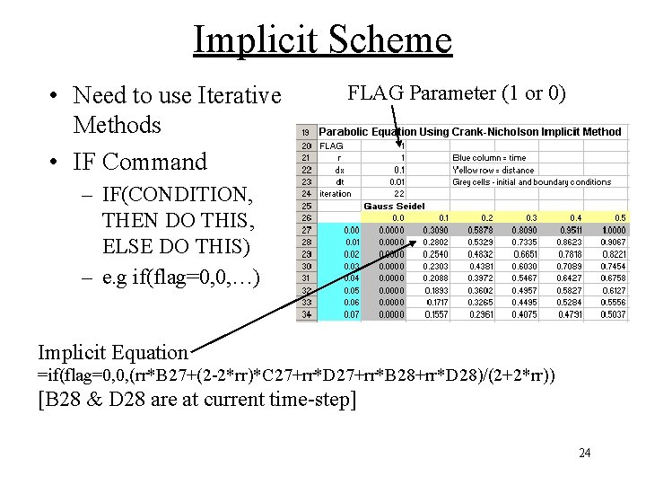
Implicit Scheme • Need to use Iterative Methods • IF Command FLAG Parameter (1 or 0) – IF(CONDITION, THEN DO THIS, ELSE DO THIS) – e. g if(flag=0, 0, …) Implicit Equation =if(flag=0, 0, (rr*B 27+(2 -2*rr)*C 27+rr*D 27+rr*B 28+rr*D 28)/(2+2*rr)) [B 28 & D 28 are at current time-step] 24