Lecture 5 Digital Image Processing Image Enhancement 1

Lecture #5 Digital Image Processing Image Enhancement 1 st Semester 2019 -2020 Dr. Abdulhussein Mohsin Abdullah Computer Science Dept. , CS & IT College, Basrah Univ.

Background q Filter term in “Digital image processing” is referred to the subimage. q There are others term to call subimage such as mask, kernel, template, or window. q The value in a filter subimage are referred as coefficients, rather than pixels.

Basics of Spatial Filtering q The concept of filtering has its roots in the use of the Fourier transform for signal processing in the so-called frequency domain. q Spatial filtering term is the filtering operations that are performed directly on the pixels of an image.

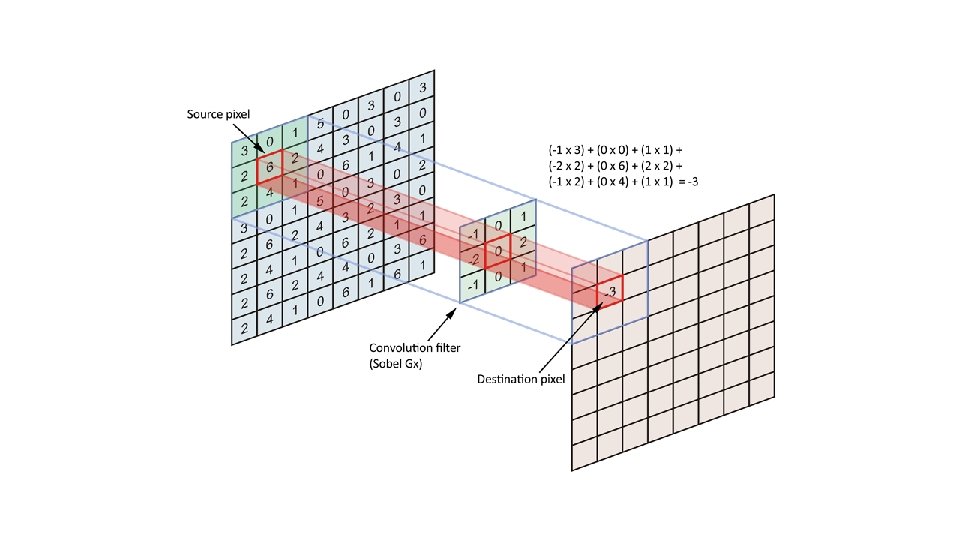
Mechanics of spatial filtering q The process consists simply of moving the filter mask from point to point in an image. q Spatial masks are used and convolved over the entire image for local enhancement (spatial filtering)

Input Image Mask

Input Image

Input Image

Input Image

Input Image

Input Image

q. At each point (x, y) the response of the filter at that point is calculated using a predefined relationship. q. The output intensity value at (x, y) depends not only on the input intensity value at (x, y) but also on the specified number of neighboring intensity values around (x, y) q. The size of the masks determines the number of neighboring pixels which influence the output value at (x, y) q. The values (coefficients) of the mask determine the nature and properties of enhancing technique

Mask Coefficients Mask The mechanics of spatial filtering w(-1, -1) w(-1, 0) w(-1, 1) w(0, -1) w(0, 0) w(0, 1) w(1, -1) w(1, 0) w(1, 1) f(x-1, y-1) f(x-1, y+1) f(x, y-1) f(x, y+1) Pixels of image section under mask f(x-1, y+1) f(x+1, y+1) For an image of size M x N and a mask of size m x n The resulting output gray level for any coordinates x and y is given by

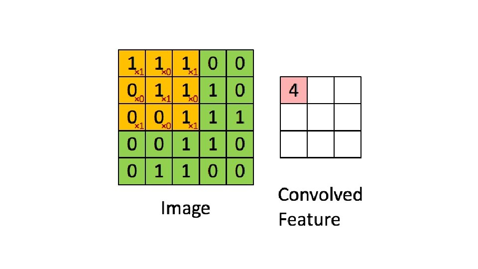
• Given the 3× 3 mask with coefficients: w 1, w 2, …, w 9 • The mask cover the pixels with gray levels: z 1, z 2, …, z 9 Z 1 Z 2 Z 3 Z 4 Z 5 Z 6 w 1 w 2 w 3 w 4 w 5 w 6 Z 7 Z 8 Z 9 w 7 w 8 w 9 Subimage Mask Coefficients • z gives the output intensity value for the processed image (to be stored in a new array) at the location of z 5 in the input image

Mask operation near the image border Problem arises when part of the mask is located outside the image plane; to handle the problem: 1. Discard the problem pixels (e. g. 512 x 512 input 510 x 510 output if mask size is 3 x 3) 2. Zero padding: expand the input image by padding zeros (512 x 512 input 514 x 514 output) • Zero padding is not good create artificial lines or edges on the border; 3. We normally use the gray levels of border pixels to fill up the expanded region (for 3 x 3 mask). For larger masks a border region equal to half of the mask size is mirrored on the expanded region.

Mask operation near the image border

Correlation vs. Convolution • The output of correlation is a weighted sum of input pixels. Need to define mask weights! output image

Correlation (linear operator) • Correlation: 1. Move the filter mask to a location 2. Compute the sum of products 3. Go to 1. a w(x, y) O f(x, y) = b Σ w(i, j ) f ( x + i, y + j ) Σ i aj b

Handling Pixels Close to Boundaries pad with zeroes 0 0 0 …………………. 0……. . 0 0 ……………. 0……………… 0

Often used in applications where we need to measure the similarity between images or parts of images (e. g. , template matching).

Convolution (linear operator) • Similar to correlation except that the mask is first flipped both horizontally and vertically. • If w(i, j) is symmetric (i. e. , w(i, j)=w(-i, -j)), then convolution is equivalent to correlation!

• Convolution: 1. Rotate the filter mask by 180 degrees 2. Correlation w(x, y) ⇥f( a x, y) = Σ b Σ i = - a j=-b w(i, j)f(x- i, y - j)

Smoothing Filters (low-pass) • Useful for reducing noise and eliminating small details. • The elements of the mask must be positive. • Mask elements sum to 1 (assuming normalization). Noise is anything in the image that we are not interested in. • Examples: – Light fluctuations – Sensor noise – Quantization effects – Finite precision

Mean (Averaging) Filter • Smoothing filters are used - Noise reduction - Smoothing of false contours - Reduction of irrelevant detail • Undesirable side effect of smoothing filters - Blur edges • The elements of the mask must be positive. • The size of the mask determines the degree of smoothing.

Consider the output pixel is positioned at the center 1 Since all weights are equal, it is called a BOX filter. 1 1 1 1 1 2 4 2 1 Weighted average give more(less) weight to pixels near (away from) the output location

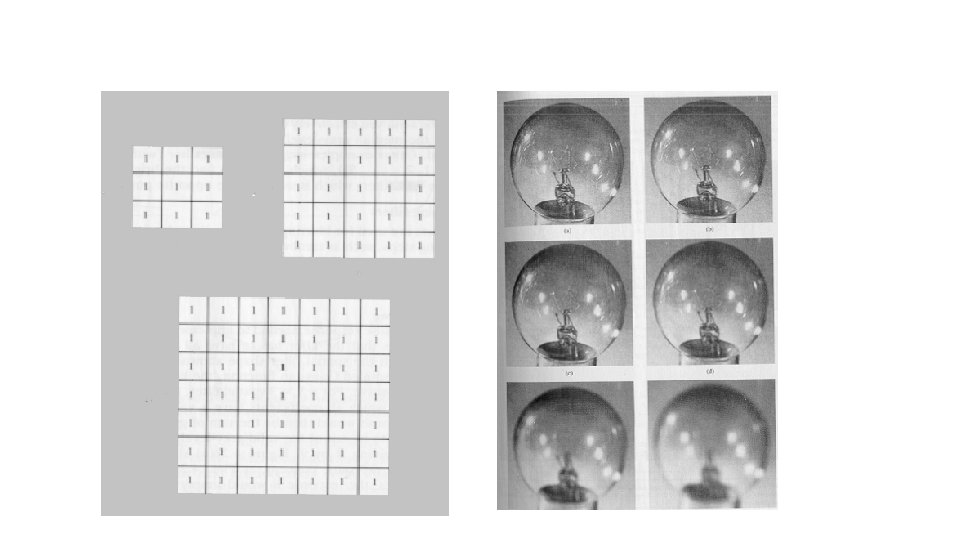
Why Averaging Reduces Noise • Intuitive explanation: variance of noise in the average is smaller than variance of the pixel noise (assuming zero-mean Gaussian noise). • Sketch of more rigorous explanation:

Spatial filtering for Smoothing • For blurring/noise reduction; • Blurring is usually used in preprocessing steps, e. g. , to remove small details from an image prior to object extraction, or to bridge small gaps in lines or curves • Equivalent to Low-pass spatial filtering in frequency domain because smaller (high frequency) details are removed based on neighborhood averaging (averaging filters)

Implementation: The simplest form of the spatial filter for averaging is a square mask (assume m×m mask) with the same coefficients 1/m 2 to preserve the gray levels (averaging). Applications: Reduce noise; smooth false contours Side effect: Edge blurring

Spatial filtering for Smoothing (example)

Spatial filtering for Smoothing (example) Original image size: 500 x 500 Smoothed by 5 x 5 box filter Smoothed by 15 x 15 box filter Smoothed by 3 x 3 box filter Smoothed by 9 x 9 box filter Smoothed by 35 x 35 box filter

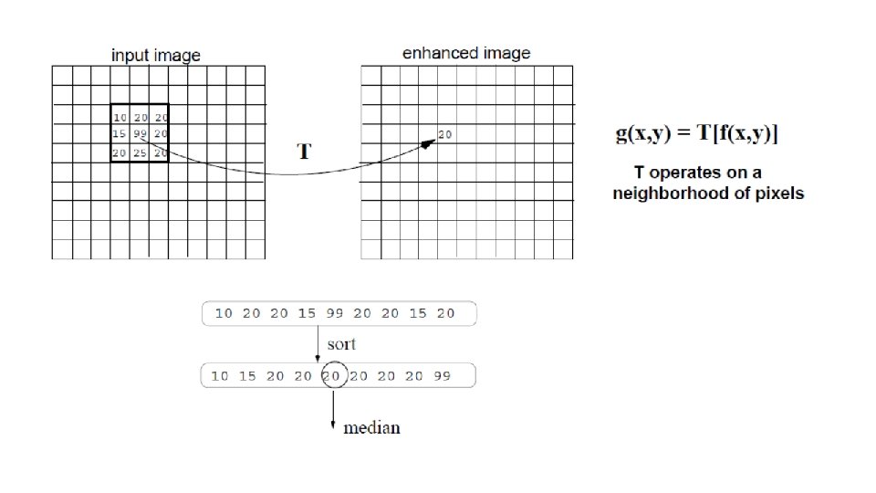
Median filter (non-linear) • Effective for removing "salt and pepper" noise (random occurrences of black and white pixels). • Replace each pixel value by the median of the gray-levels in the neighborhood of the pixels

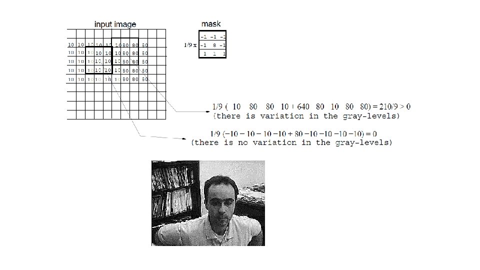
Sharpening (or High-pass) • • • It is used to emphasize the fine details of an image (has the opposite effect of smoothing). Points of high contrast can be detected by computing intensity differences in local image regions. The weights of the mask are both positive and negative. When the mask is over an area of constant or slowly varying gray level, the result of convolution will be close to zero. When gray level is varying rapidly within the neighborhood, the result of convolution will be a large number. Typically, such points form the border between different objects or scene parts (i. e. , sharpening is a precursor step to edge detection).