Lecture 5 Decision Analysis Chapter 14 Decision Environments

Lecture 5 Decision Analysis Chapter 14

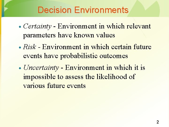
Decision Environments · Certainty - Environment in which relevant parameters have known values · Risk - Environment in which certain future events have probabilistic outcomes · Uncertainty - Environment in which it is impossible to assess the likelihood of various future events 2

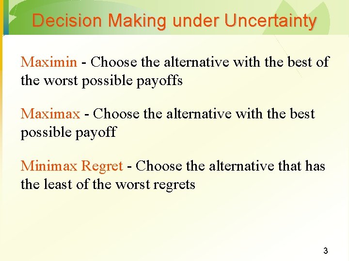
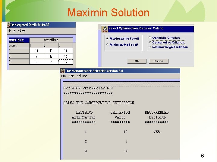
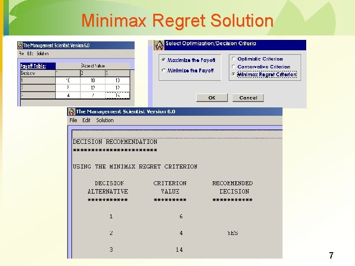
Decision Making under Uncertainty Maximin - Choose the alternative with the best of the worst possible payoffs Maximax - Choose the alternative with the best possible payoff Minimax Regret - Choose the alternative that has the least of the worst regrets 3

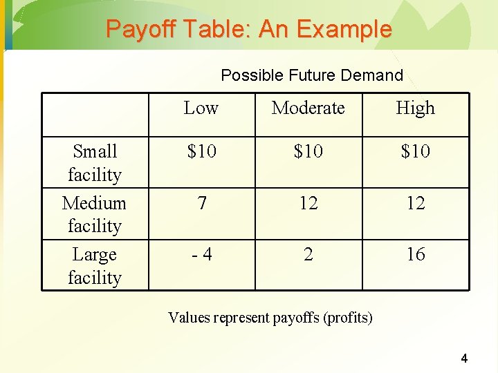
Payoff Table: An Example Possible Future Demand Small facility Medium facility Large facility Low Moderate High $10 $10 7 12 12 -4 2 16 Values represent payoffs (profits) 4

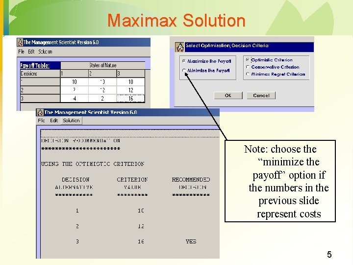
Maximax Solution Note: choose the “minimize the payoff” option if the numbers in the previous slide represent costs 5

Maximin Solution 6

Minimax Regret Solution 7

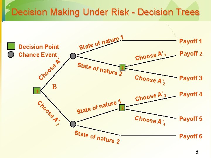
Decision Making Under Risk - Decision Trees Decision Point Chance Event ’ A e s o o h C State ture a n f o of nat 1 ho C 1 e r u t f na 2 o e t a e os St ’ 2 A State of nat ure 2 A’ 1 e s o o Ch Payoff 2 Choose A’ 2 Payoff 3 e. A s o o h C ’ 3 Payoff 4 Choose A’ 4 Payoff 5 2 ure 2 B 1 Payoff 6 8

Decision Making with Probabilities · Expected Value Approach Useful if probabilistic information regarding the states of nature is available · Expected return for each decision is calculated by summing the products of the payoff under each state of nature and the probability of the respective state of nature occurring · Decision yielding the best expected return is chosen. · 9

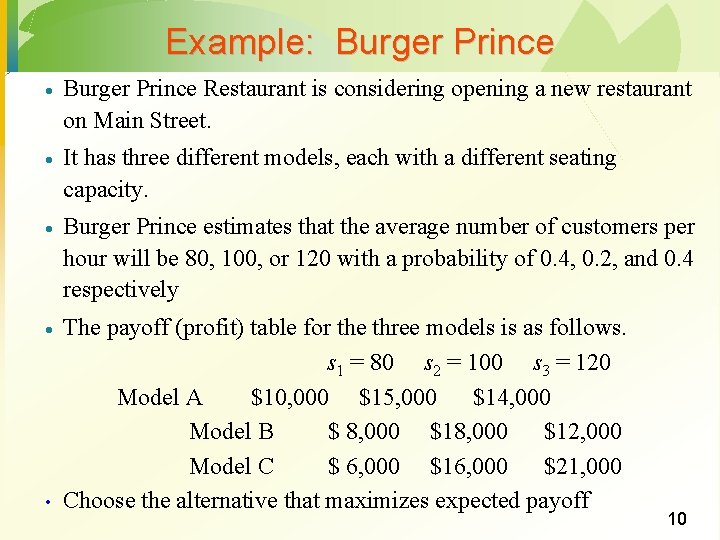
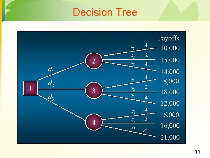
Example: Burger Prince · Burger Prince Restaurant is considering opening a new restaurant on Main Street. · It has three different models, each with a different seating capacity. · Burger Prince estimates that the average number of customers per hour will be 80, 100, or 120 with a probability of 0. 4, 0. 2, and 0. 4 respectively · The payoff (profit) table for the three models is as follows. s 1 = 80 s 2 = 100 s 3 = 120 Model A $10, 000 $15, 000 $14, 000 Model B $ 8, 000 $12, 000 Model C $ 6, 000 $16, 000 $21, 000 Choose the alternative that maximizes expected payoff • 10

Decision Tree d 1 1 d 2 d 3 2 3 4 s 1 s 2 s 3 . 4. 2. 4 Payoffs 10, 000 15, 000 14, 000 8, 000 12, 000 6, 000 16, 000 21, 000 11

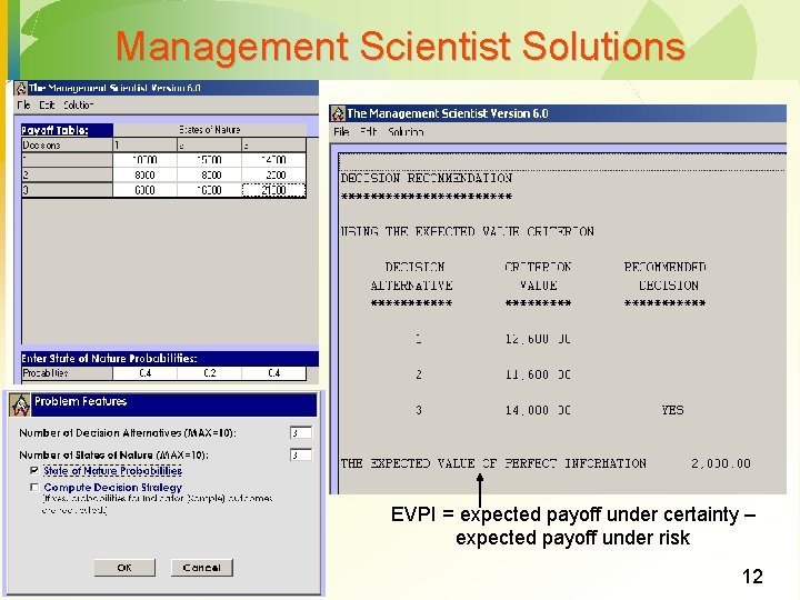
Management Scientist Solutions EVPI = expected payoff under certainty – expected payoff under risk 12

Lecture 5 Inventory Management Chapter 11

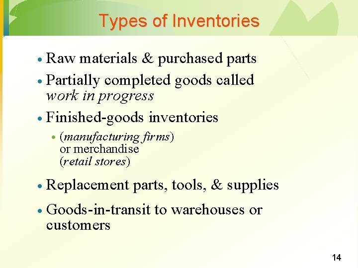
Types of Inventories Raw materials & purchased parts · Partially completed goods called work in progress · Finished-goods inventories · · (manufacturing firms) or merchandise (retail stores) · Replacement parts, tools, & supplies · Goods-in-transit to warehouses or customers 14

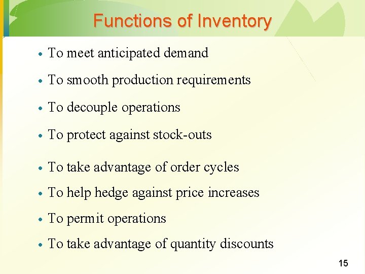
Functions of Inventory · To meet anticipated demand · To smooth production requirements · To decouple operations · To protect against stock-outs · To take advantage of order cycles · To help hedge against price increases · To permit operations · To take advantage of quantity discounts 15

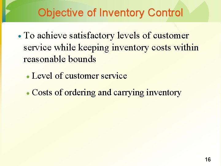
Objective of Inventory Control · To achieve satisfactory levels of customer service while keeping inventory costs within reasonable bounds · Level of customer service · Costs of ordering and carrying inventory 16

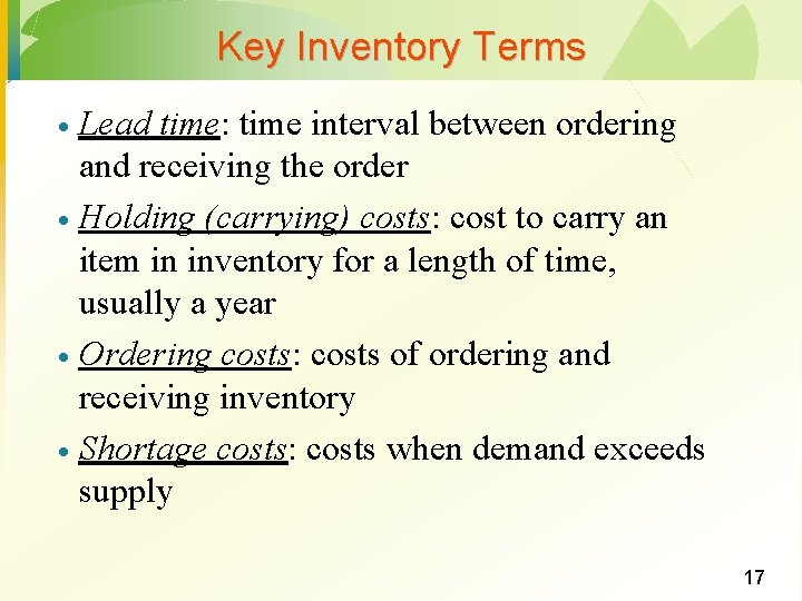
Key Inventory Terms Lead time: time interval between ordering and receiving the order · Holding (carrying) costs: cost to carry an item in inventory for a length of time, usually a year · Ordering costs: costs of ordering and receiving inventory · Shortage costs: costs when demand exceeds supply · 17

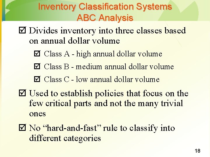
Inventory Classification Systems ABC Analysis þ Divides inventory into three classes based on annual dollar volume þ Class A - high annual dollar volume þ Class B - medium annual dollar volume þ Class C - low annual dollar volume þ Used to establish policies that focus on the few critical parts and not the many trivial ones þ No “hard-and-fast” rule to classify into different categories 18

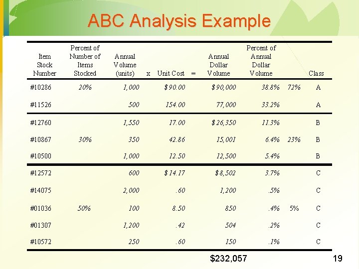
ABC Analysis Example Item Stock Number #10286 Percent of Number of Items Stocked x Unit Cost = Annual Dollar Volume Class 1, 000 $ 90, 000 38. 8% #11526 500 154. 00 77, 000 33. 2% A #12760 1, 550 17. 00 $ 26, 350 11. 3% B 350 42. 86 15, 001 6. 4% #10500 1, 000 12. 50 12, 500 5. 4% B #12572 600 $ 14. 17 $ 8, 502 3. 7% C #14075 2, 000 . 60 1, 200 . 5% C 100 8. 50 850 . 4% #01307 1, 200 . 42 504 . 2% C #10572 250 . 60 150 . 1% C #10867 #01036 20% Annual Volume (units) Percent of Annual Dollar Volume 30% 50% $232, 057 72% 23% 5% A B C 19

Economic Order Quantity Models · Economic order quantity (EOQ) model · Quantity discount model · Economic production model (EPQ) 20

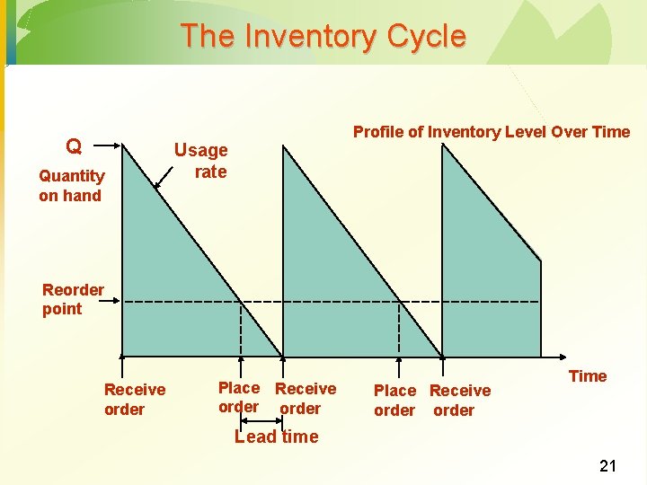
The Inventory Cycle Q Quantity on hand Profile of Inventory Level Over Time Usage rate Reorder point Receive order Place Receive order Time Lead time 21

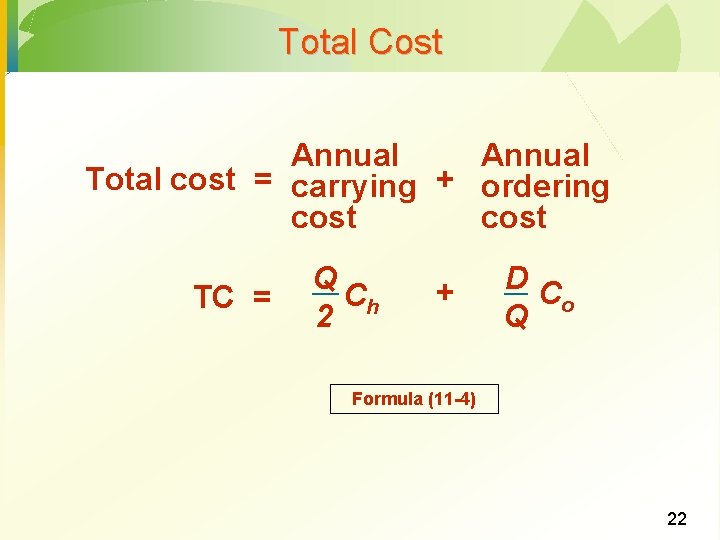
Total Cost Annual Total cost = carrying + ordering cost TC = Q Ch 2 + DC Q o Formula (11 -4) 22

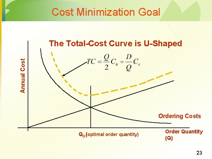
Cost Minimization Goal Annual Cost The Total-Cost Curve is U-Shaped Ordering Costs QO (optimal order quantity) Order Quantity (Q) 23

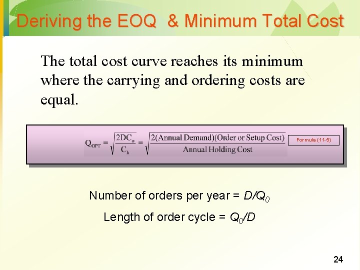
Deriving the EOQ & Minimum Total Cost The total cost curve reaches its minimum where the carrying and ordering costs are equal. Formula (11 -5) Number of orders per year = D/Q 0 Length of order cycle = Q 0/D 24

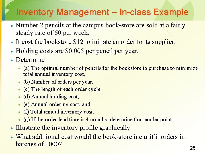
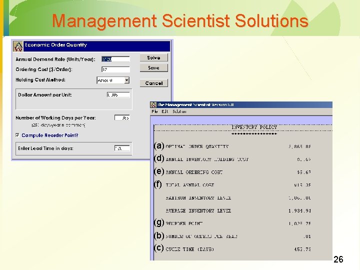
Inventory Management – In-class Example · · Number 2 pencils at the campus book-store are sold at a fairly steady rate of 60 per week. It cost the bookstore $12 to initiate an order to its supplier. Holding costs are $0. 005 per pencil per year. Determine · · · · · (a) The optimal number of pencils for the bookstore to purchase to minimize total annual inventory cost, (b) Number of orders per year, (c) The length of each order cycle, (d) Annual holding cost, (e) Annual ordering cost, and (f) Total annual inventory cost. (g) If the order lead time is 4 months, determine the reorder point. Illustrate the inventory profile graphically. What additional cost would the book-store incur if it orders in batches of 1000? 25

Management Scientist Solutions (a) (d) (e) (f) (g) (b) (c) 26

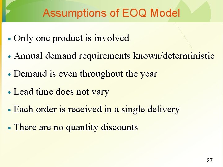
Assumptions of EOQ Model · Only one product is involved · Annual demand requirements known/deterministic · Demand is even throughout the year · Lead time does not vary · Each order is received in a single delivery · There are no quantity discounts 27

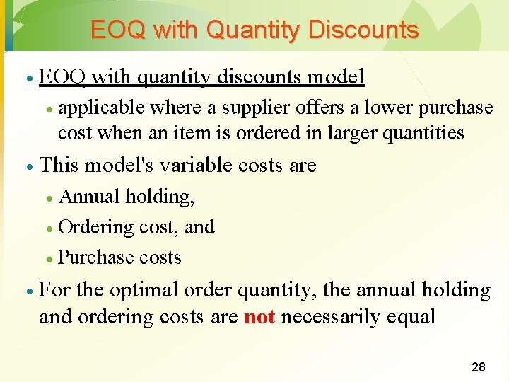
EOQ with Quantity Discounts · EOQ with quantity discounts model · · applicable where a supplier offers a lower purchase cost when an item is ordered in larger quantities This model's variable costs are Annual holding, · Ordering cost, and · Purchase costs · · For the optimal order quantity, the annual holding and ordering costs are not necessarily equal 28

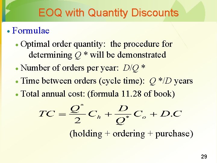
EOQ with Quantity Discounts · Formulae Optimal order quantity: the procedure for determining Q * will be demonstrated · Number of orders per year: D/Q * · Time between orders (cycle time): Q */D years · Total annual cost: (formula 11. 28 of book) · (holding + ordering + purchase) 29

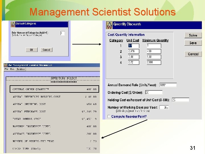
Example – EOQ with Quantity Discount · · · · Walgreens carries Fuji 400 X instant print film The film normally costs Walgreens $3. 20 per roll Walgreens sells each roll for $5. 25 Walgreens's average sales are 21 rolls per week Walgreens’s annual inventory holding cost rate is 25% It costs Walgreens $20 to place an order with Fujifilm, USA Fujifilm offers the following discount scheme to Walgreens · 7% discount on orders of 400 rolls or more · 10% discount for 900 rolls or more, and · 15% discount for 2000 rolls or more Determine Walgreen’s optimal order quantity 30

Management Scientist Solutions 31