Lecture 5 Constraint Satisfaction Problems CPEN 405 Artificial

Lecture 5: Constraint Satisfaction Problems CPEN 405: Artificial Intelligence Instructor: Robert Sowah, Ph. D

Outline • What is a CSP • Backtracking for CSP • Local search for CSPs • Problem structure and decomposition

Constraint Satisfaction Problems • What is a CSP? – Finite set of variables V 1, V 2, …, Vn • Nonempty domain of possible values for each variable DV 1, DV 2, … DVn – Finite set of constraints C 1, C 2, …, Cm • Each constraint Ci limits the values that variables can take, – e. g. , V 1 ≠ V 2 • A state is defined as an assignment of values to some or all variables. • Consistent assignment – assignment does not violate the constraints • CSP benefits – Standard representation pattern – Generic goal and successor functions – Generic heuristics (no domain specific expertise).

CSPs (continued) • An assignment is complete when every variable is mentioned. • A solution to a CSP is a complete assignment that satisfies all constraints. • Some CSPs require a solution that maximizes an objective function. • Examples of Applications: – – – Scheduling the time of observations on the Hubble Space Telescope Airline schedules Cryptography Computer vision -> image interpretation Scheduling your MS or Ph. D thesis exam

CSP example: map coloring • Variables: WA, NT, Q, NSW, V, SA, T • Domains: Di={red, green, blue} • Constraints: adjacent regions must have different colors. • E. g. WA NT

CSP example: map coloring • Solutions are assignments satisfying all constraints, e. g. {WA=red, NT=green, Q=red, NSW=green, V=red, SA=blue, T=green}

Graph coloring • More general problem than map coloring • Planar graph = graph in the 2 d-plane with no edge crossings • Guthrie’s conjecture (1852) Every planar graph can be colored with 4 colors or less – Proved (using a computer) in 1977 (Appel and Haken)

Constraint graphs • Constraint graph: • nodes are variables • arcs are binary constraints • Graph can be used to simplify search e. g. Tasmania is an independent subproblem (will return to graph structure later)

Varieties of CSPs • Discrete variables – Finite domains; size d O(dn) complete assignments. • E. g. Boolean CSPs: Boolean satisfiability (NP-complete). – Infinite domains (integers, strings, etc. ) • • • E. g. job scheduling, variables are start/end days for each job Need a constraint language e. g Start. Job 1 +5 ≤ Start. Job 3. Infinitely many solutions Linear constraints: solvable Nonlinear: no general algorithm • Continuous variables – e. g. building an airline schedule or class schedule. – Linear constraints solvable in polynomial time by LP methods.

Varieties of constraints • Unary constraints involve a single variable. – e. g. SA green • Binary constraints involve pairs of variables. – e. g. SA WA • Higher-order constraints involve 3 or more variables. – Professors A, B, and C cannot be on a committee together – Can always be represented by multiple binary constraints • Preference (soft constraints) – e. g. red is better than green often can be represented by a cost for each variable assignment – combination of optimization with CSPs

CSP Example: Cryptharithmetic puzzle

CSP as a standard search problem • A CSP can easily be expressed as a standard search problem. • Incremental formulation – Initial State: the empty assignment {} – Successor function: Assign a value to any unassigned variable provided that it does not violate a constraint – Goal test: the current assignment is complete (by construction its consistent) – Path cost: constant cost for every step (not really relevant) • Can also use complete-state formulation – Local search techniques (Chapter 4) tend to work well

CSP as a standard search problem • Solution is found at depth n (if there are n variables). • Consider using BFS – Branching factor b at the top level is nd – At next level is (n-1)d – …. • end up with n!dn leaves even though there are only dn complete assignments!

Commutativity • CSPs are commutative. – The order of any given set of actions has no effect on the outcome. – Example: choose colors for Australian territories one at a time • [WA=red then NT=green] same as [NT=green then WA=red] • All CSP search algorithms can generate successors by considering assignments for only a single variable at each node in the search tree there are dn leaves (will need to figure out later which variable to assign a value to at each node)

Backtracking search • Similar to Depth-first search • Chooses values for one variable at a time and backtracks when a variable has no legal values left to assign. • Uninformed algorithm – No good general performance (see table p. 143)

Backtracking example

Comparison of CSP algorithms on different problems Median number of consistency checks over 5 runs to solve problem Parentheses -> no solution found USA: 4 coloring n-queens: n = 2 to 50 Zebra: see exercise 5. 13

Improving CSP efficiency • Previous improvements on uninformed search introduce heuristics • For CSPS, general-purpose methods can give large gains in speed, e. g. , – – Which variable should be assigned next? In what order should its values be tried? Can we detect inevitable failure early? Can we take advantage of problem structure? Note: CSPs are somewhat generic in their formulation, and so the heuristics are more general compared to methods in Chapter 4

Minimum remaining values (MRV) var SELECT-UNASSIGNED-VARIABLE(VARIABLES[csp], assignment, csp) • A. k. a. most constrained variable heuristic • Heuristic Rule: choose variable with the fewest legal moves – e. g. , will immediately detect failure if X has no legal values

Degree heuristic for the initial variable • Heuristic Rule: select variable that is involved in the largest number of constraints on other unassigned variables. • Degree heuristic can be useful as a tie breaker. • In what order should a variable’s values be tried?

Least constraining value for value-ordering • Least constraining value heuristic • Heuristic Rule: given a variable choose the least constraining value – leaves the maximum flexibility for subsequent variable assignments

Forward checking • Can we detect inevitable failure early? – And avoid it later? • Forward checking idea: keep track of remaining legal values for unassigned variables. • Terminate search when any variable has no legal values.

Forward checking • Assign {WA=red} • Effects on other variables connected by constraints to WA – – NT can no longer be red SA can no longer be red

Forward checking • Assign {Q=green} • Effects on other variables connected by constraints with WA – – – • NT can no longer be green NSW can no longer be green SA can no longer be green MRV heuristic would automatically select NT or SA next

Forward checking • If V is assigned blue • Effects on other variables connected by constraints with WA – NSW can no longer be blue – SA is empty • FC has detected that partial assignment is inconsistent with the constraints and backtracking can occur.

Example: 4 -Queens Problem 1 2 3 4 X 1 {1, 2, 3, 4} X 2 {1, 2, 3, 4} X 3 {1, 2, 3, 4} X 4 {1, 2, 3, 4} 1 2 3 4

Example: 4 -Queens Problem 1 2 3 4 X 1 {1, 2, 3, 4} X 2 { , , 3, 4} X 3 { , 2, , 4} X 4 { , 2, 3, } 1 2 3 4

Example: 4 -Queens Problem 1 2 3 4 X 1 {1, 2, 3, 4} X 2 { , , 3, 4} X 3 { , , , } X 4 { , , 3, } 1 2 3 4

Example: 4 -Queens Problem 1 2 3 4 X 1 {1, 2, 3, 4} X 2 { , , , 4} X 3 { , 2, , 4} X 4 { , 2, 3, } 1 2 3 4

Example: 4 -Queens Problem 1 2 3 4 X 1 {1, 2, 3, 4} X 2 { , , , 4} X 3 { , 2, , } X 4 { , , 3, } 1 2 3 4

Example: 4 -Queens Problem 1 2 3 4 X 1 {1, 2, 3, 4} X 2 { , , 3, 4} X 3 { , 2, , } X 4 { , , , } 1 2 3 4

Problem Consider the constraint graph on the right. b The domain for every variable is [1, 2, 3, 4]. There are 2 unary constraints: - variable “a” cannot take values 3 and 4. - variable “b” cannot take value 4. There are 8 binary constraints stating that variables connected by an edge cannot have the same value. Find a solution for this CSP by using the following heuristics: minimum value heuristic, degree heuristic, forward checking. a c d e

Problem Consider the constraint graph on the right. b The domain for every variable is [1, 2, 3, 4]. There are 2 unary constraints: - variable “a” cannot take values 3 and 4. - variable “b” cannot take value 4. There are 8 binary constraints stating that variables connected by an edge cannot have the same value. Find a solution for this CSP by using the following heuristics: minimum value heuristic, degree heuristic, forward checking. MVH FC+MVH+DH FC+MVH FC a=1 (for example) b=2 c=3 d=4 e=1 a c d e

Comparison of CSP algorithms on different problems Median number of consistency checks over 5 runs to solve problem Parentheses -> no solution found USA: 4 coloring n-queens: n = 2 to 50 Zebra: see exercise 5. 13

Constraint propagation • Solving CSPs with combination of heuristics plus forward checking is more efficient than either approach alone • FC checking does not detect all failures. – E. g. , NT and SA cannot be blue

Constraint propagation • Techniques like CP and FC are in effect eliminating parts of the search space – Somewhat complementary to search • Constraint propagation goes further than FC by repeatedly enforcing constraints locally – Needs to be faster than actually searching to be effective • Arc-consistency (AC) is a systematic procedure for constraing propagation

Arc consistency • An Arc X Y is consistent if for every value x of X there is some value y consistent with x (note that this is a directed property) • Consider state of search after WA and Q are assigned: SA NSW is consistent if SA=blue and NSW=red

Arc consistency • X Y is consistent if for every value x of X there is some value y consistent with x • NSW SA is consistent if NSW=red and SA=blue NSW=blue and SA=? ? ?

Arc consistency • Can enforce arc-consistency: Arc can be made consistent by removing blue from NSW • Continue to propagate constraints…. – Check V NSW – Not consistent for V = red – Remove red from V

Arc consistency • Continue to propagate constraints…. • SA NT is not consistent – and cannot be made consistent • Arc consistency detects failure earlier than FC

Arc consistency checking • Can be run as a preprocessor or after each assignment – Or as preprocessing before search starts • AC must be run repeatedly until no inconsistency remains • Trade-off – Requires some overhead to do, but generally more effective than direct search – In effect it can eliminate large (inconsistent) parts of the state space more effectively than search can • Need a systematic method for arc-checking – If X loses a value, neighbors of X need to be rechecked: i. e. incoming arcs can become inconsistent again (outgoing arcs will stay consistent).

Arc consistency algorithm (AC-3) function AC-3(csp) return the CSP, possibly with reduced domains inputs: csp, a binary csp with variables {X 1, X 2, …, Xn} local variables: queue, a queue of arcs initially the arcs in csp while queue is not empty do (Xi, Xj) REMOVE-FIRST(queue) if REMOVE-INCONSISTENT-VALUES(Xi, Xj) then for each Xk in NEIGHBORS[Xi ] do add (Xi, Xj) to queue function REMOVE-INCONSISTENT-VALUES(Xi, Xj) return true iff we remove a value removed false for each x in DOMAIN[Xi] do if no value y in DOMAIN[Xi] allows (x, y) to satisfy the constraints between Xi and Xj then delete x from DOMAIN[Xi]; removed true return removed (from Mackworth, 1977)

Another problem to try [R, B, G] [R] [R, B, G] Use all heuristics including arc-propagation to solve this problem.

Complexity of AC-3 • A binary CSP has at most n 2 arcs • Each arc can be inserted in the queue d times (worst case) – (X, Y): only d values of X to delete • Consistency of an arc can be checked in O(d 2) time • Complexity is O(n 2 d 3)

Arc-consistency as message-passing • This is a propagation algorithm. It’s like sending messages to neighbors on the graph. How do we schedule these messages? • Every time a domain changes, all incoming messages need to be resent. Repeat until convergence no message will change any domains. • Since we only remove values from domains when they can never be part of a solution, an empty domain means no solution possible at all back out of that branch. • Forward checking is simply sending messages into a variable that just got its value assigned. First step of arc-consistency.

K-consistency • Arc consistency does not detect all inconsistencies: – Partial assignment {WA=red, NSW=red} is inconsistent. • Stronger forms of propagation can be defined using the notion of kconsistency. • A CSP is k-consistent if for any set of k-1 variables and for any consistent assignment to those variables, a consistent value can always be assigned to any kth variable. – E. g. 1 -consistency = node-consistency – E. g. 2 -consistency = arc-consistency – E. g. 3 -consistency = path-consistency • Strongly k-consistent: – k-consistent for all values {k, k-1, … 2, 1}

Trade-offs • Running stronger consistency checks… – Takes more time – But will reduce branching factor and detect more inconsistent partial assignments – No “free lunch” • In worst case n-consistency takes exponential time

Further improvements • Checking special constraints – Checking Alldif(…) constraint • E. g. {WA=red, NSW=red} – Checking Atmost(…) constraint • Bounds propagation for larger value domains • Intelligent backtracking – Standard form is chronological backtracking i. e. try different value for preceding variable. – More intelligent, backtrack to conflict set. • Set of variables that caused the failure or set of previously assigned variables that are connected to X by constraints. • Backjumping moves back to most recent element of the conflict set. • Forward checking can be used to determine conflict set.

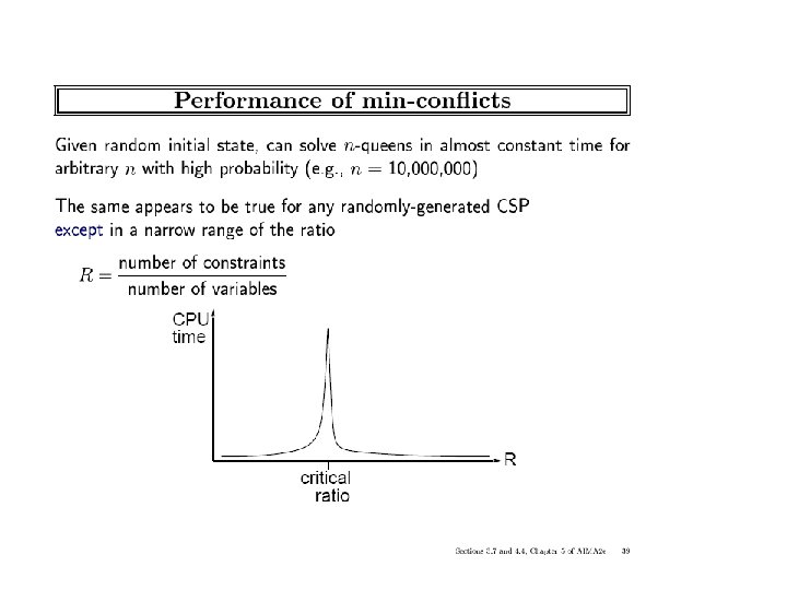
Local search for CSPs • Use complete-state representation – Initial state = all variables assigned values – Successor states = change 1 (or more) values • For – – – CSPs allow states with unsatisfied constraints (unlike backtracking) operators reassign variable values hill-climbing with n-queens is an example • Variable selection: randomly select any conflicted variable • Value selection: min-conflicts heuristic – Select new value that results in a minimum number of conflicts with the other variables

Local search for CSP function MIN-CONFLICTS(csp, max_steps) return solution or failure inputs: csp, a constraint satisfaction problem max_steps, the number of steps allowed before giving up current an initial complete assignment for csp for i = 1 to max_steps do if current is a solution for csp then return current var a randomly chosen, conflicted variable from VARIABLES[csp] value the value v for var that minimize CONFLICTS(var, v, current, csp) set var = value in current return failure

Min-conflicts example 1 h=5 h=3 Use of min-conflicts heuristic in hill-climbing. h=1

Min-conflicts example 2 • A two-step solution for an 8 -queens problem using min-conflicts heuristic • At each stage a queen is chosen for reassignment in its column • The algorithm moves the queen to the min-conflict square breaking ties randomly.

Comparison of CSP algorithms on different problems Median number of consistency checks over 5 runs to solve problem Parentheses -> no solution found USA: 4 coloring n-queens: n = 2 to 50 Zebra: see exercise 5. 13

Advantages of local search • Local search can be particularly useful in an online setting – Airline schedule example • E. g. , mechanical problems require than 1 plane is taken out of service • Can locally search for another “close” solution in state-space • Much better (and faster) in practice than finding an entirely new schedule • The runtime of min-conflicts is roughly independent of problem size. – Can solve the millions-queen problem in roughly 50 steps. – Why? • n-queens is easy for local search because of the relatively high density of solutions in state-space

Graph structure and problem complexity • Solving disconnected subproblems – Suppose each subproblem has c variables out of a total of n. – Worst case solution cost is O(n/c dc), i. e. linear in n • Instead of O(d n), exponential in n • E. g. n= 80, c= 20, d=2 – – 280 = 4 billion years at 1 million nodes/sec. 4 * 220=. 4 second at 1 million nodes/sec

Tree-structured CSPs • Theorem: – if a constraint graph has no loops then the CSP can be solved in O(nd 2) time – linear in the number of variables! • Compare difference with general CSP, where worst case is O(d n)

Algorithm for Solving Tree-structured CSPs – Choose some variable as root, order variables from root to leaves such that every node’s parent precedes it in the ordering. • Label variables from X 1 to Xn) • Every variable now has 1 parent – Backward Pass • For j from n down to 2, apply arc consistency to arc [Parent(Xj), Xj) ] • Remove values from Parent(Xj) if needed – Forward Pass • For j from 1 to n assign Xj consistently with Parent(Xj )

Tree CSP Example G B

Tree CSP Example Backward Pass (constraint propagation) B R G B

Tree CSP Example Backward Pass (constraint propagation) Forward Pass (assignment) B R G B B G B R G G R R R G G B B

Tree CSP complexity • Backward pass – n arc checks – Each has complexity d 2 at worst • Forward pass – n variable assignments, O(nd) Overall complexity is O(nd 2) Algorithm works because if the backward pass succeeds, then every variable by definition has a legal assignment in the forward pass

What about non-tree CSPs? • General idea is to convert the graph to a tree 2 general approaches 1. Assign values to specific variables (Cycle Cutset method) 2. Construct a tree-decomposition of the graph - Connected subproblems (subgraphs) form a tree structure

Cycle-cutset conditioning • Choose a subset S of variables from the graph so that graph without S is a tree – S = “cycle cutset” • For each possible consistent assignment for S – Remove any inconsistent values from remaining variables that are inconsistent with S – Use tree-structured CSP to solve the remaining tree-structure • If it has a solution, return it along with S • If not, continue to try other assignments for S

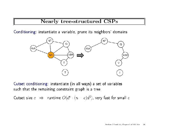
Finding the optimal cutset • If c is small, this technique works very well • However, finding smallest cycle cutset is NP-hard – But there are good approximation algorithms

Tree Decompositions

Rules for a Tree Decomposition • Every variable appears in at least one of the subproblems • If two variables are connected in the original problem, they must appear together (with the constraint) in at least one subproblem • If a variable appears in two subproblems, it must appear in each node on the path.

Tree Decomposition Algorithm • View each subproblem as a “super-variable” – Domain = set of solutions for the subproblem – Obtained by running a CSP on each subproblem – E. g. , 6 solutions for 3 fully connected variables in map problem • Now use the tree CSP algorithm to solve the constraints connecting the subproblems – Declare a subproblem a root node, create tree – Backward and forward passes • Example of “divide and conquer” strategy

Complexity of Tree Decomposition • Many possible tree decompositions for a graph • Tree-width of a tree decomposition = 1 less than the size of the largest subproblem • Tree-width of a graph = minimum tree width • If a graph has tree width w, then solving the CSP can be done in O(n dw+1) time (why? ) – CSPs of bounded tree-width are solvable in polynomial time • Finding the optimal tree-width of a graph is NP-hard, but good heuristics exist.

Summary • CSPs – special kind of problem: states defined by values of a fixed set of variables, goal test defined by constraints on variable values • Backtracking=depth-first search with one variable assigned per node • Heuristics – Variable ordering and value selection heuristics help significantly • Constraint propagation does additional work to constrain values and detect inconsistencies – Works effectively when combined with heuristics • Iterative min-conflicts is often effective in practice. • Graph structure of CSPs determines problem complexity – e. g. , tree structured CSPs can be solved in linear time.