Lecture 5 Collocations Chapter 5 of Manning and
- Slides: 31

Lecture 5: Collocations (Chapter 5 of Manning and Schutze) Wen-Hsiang Lu (盧文祥) Department of Computer Science and Information Engineering, National Cheng Kung University 2014/03/10 (Slides from Dr. Mary P. Harper, http: //min. ecn. purdue. edu/~ee 669/) Fall 2001 EE 669: Natural Language Processing 1

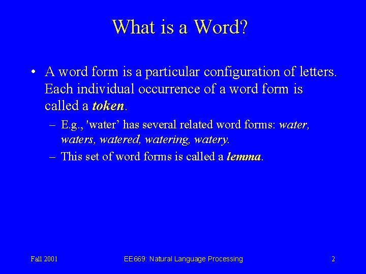
What is a Word? • A word form is a particular configuration of letters. Each individual occurrence of a word form is called a token. – E. g. , 'water’ has several related word forms: water, waters, watered, watering, watery. – This set of word forms is called a lemma. Fall 2001 EE 669: Natural Language Processing 2

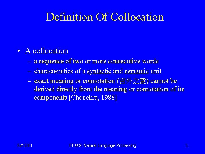
Definition Of Collocation • A collocation – a sequence of two or more consecutive words – characteristics of a syntactic and semantic unit – exact meaning or connotation (言外之意) cannot be derived directly from the meaning or connotation of its components [Chouekra, 1988] Fall 2001 EE 669: Natural Language Processing 3

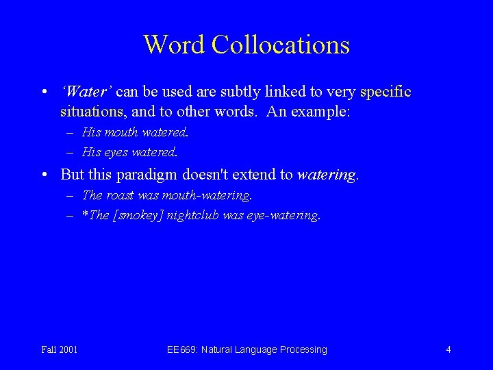
Word Collocations • ‘Water’ can be used are subtly linked to very specific situations, and to other words. An example: – His mouth watered. – His eyes watered. • But this paradigm doesn't extend to watering. – The roast was mouth-watering. – *The [smokey] nightclub was eye-watering. Fall 2001 EE 669: Natural Language Processing 4

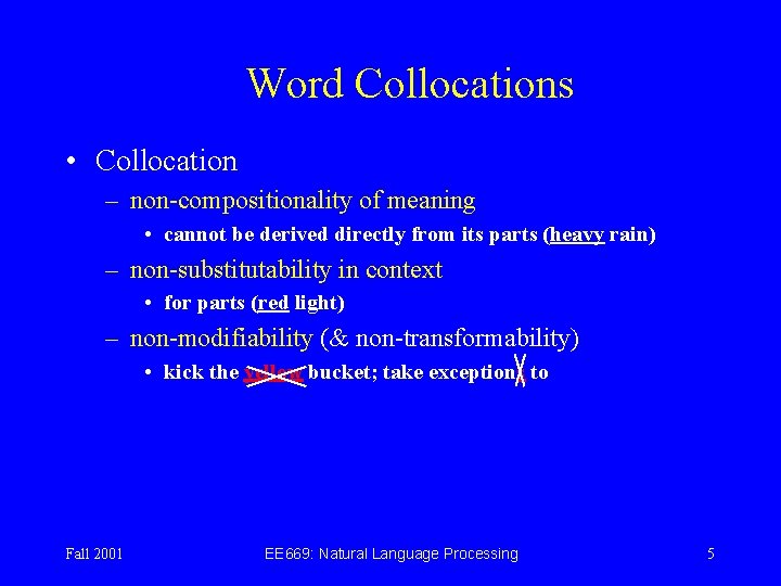
Word Collocations • Collocation – non-compositionality of meaning • cannot be derived directly from its parts (heavy rain) – non-substitutability in context • for parts (red light) – non-modifiability (& non-transformability) • kick the yellow bucket; take exceptions to Fall 2001 EE 669: Natural Language Processing 5

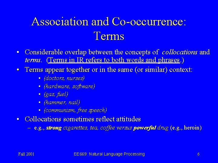
Association and Co-occurrence: Terms • Considerable overlap between the concepts of collocations and terms. (Terms in IR refers to both words and phrases. ) • Terms appear together or in the same (or similar) context: • • • (doctors, nurses) (hardware, software) (gas, fuel) (hammer, nail) (communism, free speech) • Collocations sometimes reflect attitudes – e. g. , strong cigarettes, tea, coffee versus powerful drug (e. g. , heroin) Fall 2001 EE 669: Natural Language Processing 6

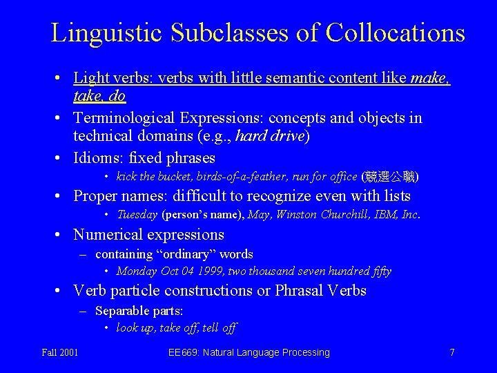
Linguistic Subclasses of Collocations • Light verbs: verbs with little semantic content like make, take, do • Terminological Expressions: concepts and objects in technical domains (e. g. , hard drive) • Idioms: fixed phrases • kick the bucket, birds-of-a-feather, run for office (競選公職) • Proper names: difficult to recognize even with lists • Tuesday (person’s name), May, Winston Churchill, IBM, Inc. • Numerical expressions – containing “ordinary” words • Monday Oct 04 1999, two thousand seven hundred fifty • Verb particle constructions or Phrasal Verbs – Separable parts: • look up, take off, tell off Fall 2001 EE 669: Natural Language Processing 7

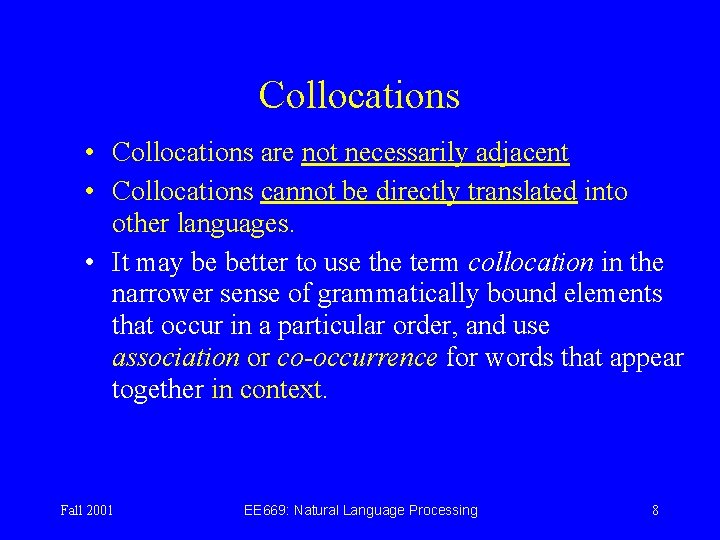
Collocations • Collocations are not necessarily adjacent • Collocations cannot be directly translated into other languages. • It may be better to use the term collocation in the narrower sense of grammatically bound elements that occur in a particular order, and use association or co-occurrence for words that appear together in context. Fall 2001 EE 669: Natural Language Processing 8

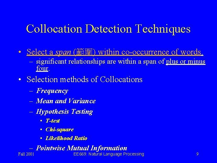
Collocation Detection Techniques • Select a span (範圍) within co-occurrence of words. – significant relationships are within a span of plus or minus four. • Selection methods of Collocations – Frequency – Mean and Variance – Hypothesis Testing • T-test • Chi-square • Likelihood Ratio – Pointwise Mutual Information Fall 2001 EE 669: Natural Language Processing 9

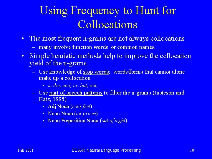
Using Frequency to Hunt for Collocations • The most frequent n-grams are not always collocations – many involve function words or common names. • Simple heuristic methods help to improve the collocation yield of the n-grams. – Use knowledge of stop words; words/forms that cannot alone make up a collocation • a, the, and, or, but, not, … – Use part of speech patterns to filter the n-grams (Justeson and Katz, 1995) • Adj Noun (cold feet) • Noun (oil prices) • Noun Preposition Noun (out of sight) Fall 2001 EE 669: Natural Language Processing 10

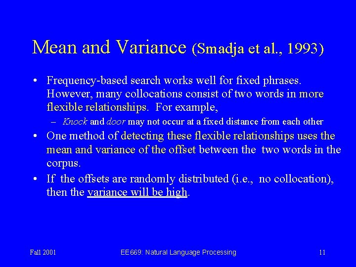
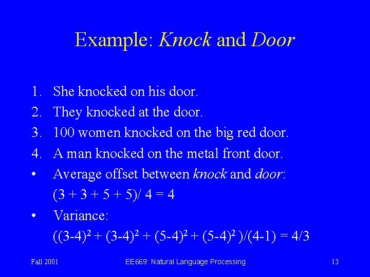
Mean and Variance (Smadja et al. , 1993) • Frequency-based search works well for fixed phrases. However, many collocations consist of two words in more flexible relationships. For example, – Knock and door may not occur at a fixed distance from each other • One method of detecting these flexible relationships uses the mean and variance of the offset between the two words in the corpus. • If the offsets are randomly distributed (i. e. , no collocation), then the variance will be high. Fall 2001 EE 669: Natural Language Processing 11

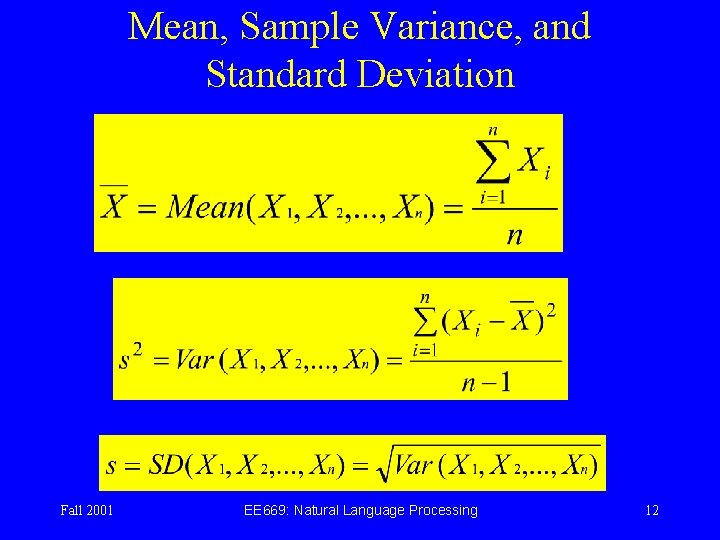
Mean, Sample Variance, and Standard Deviation Fall 2001 EE 669: Natural Language Processing 12

Example: Knock and Door 1. 2. 3. 4. • • She knocked on his door. They knocked at the door. 100 women knocked on the big red door. A man knocked on the metal front door. Average offset between knock and door: (3 + 5 + 5)/ 4 = 4 Variance: ((3 -4)2 + (5 -4)2 )/(4 -1) = 4/3 Fall 2001 EE 669: Natural Language Processing 13

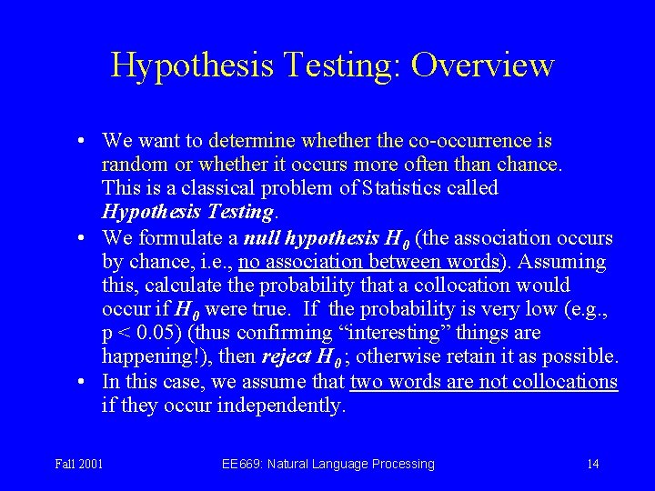
Hypothesis Testing: Overview • We want to determine whether the co-occurrence is random or whether it occurs more often than chance. This is a classical problem of Statistics called Hypothesis Testing. • We formulate a null hypothesis H 0 (the association occurs by chance, i. e. , no association between words). Assuming this, calculate the probability that a collocation would occur if H 0 were true. If the probability is very low (e. g. , p < 0. 05) (thus confirming “interesting” things are happening!), then reject H 0 ; otherwise retain it as possible. • In this case, we assume that two words are not collocations if they occur independently. Fall 2001 EE 669: Natural Language Processing 14

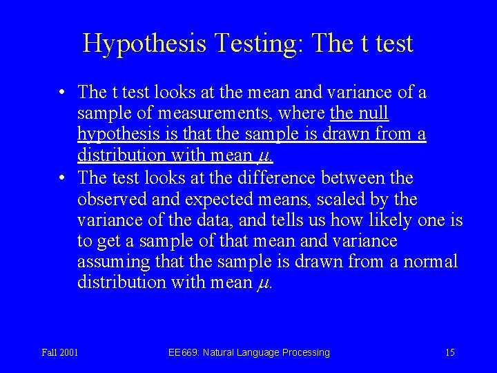
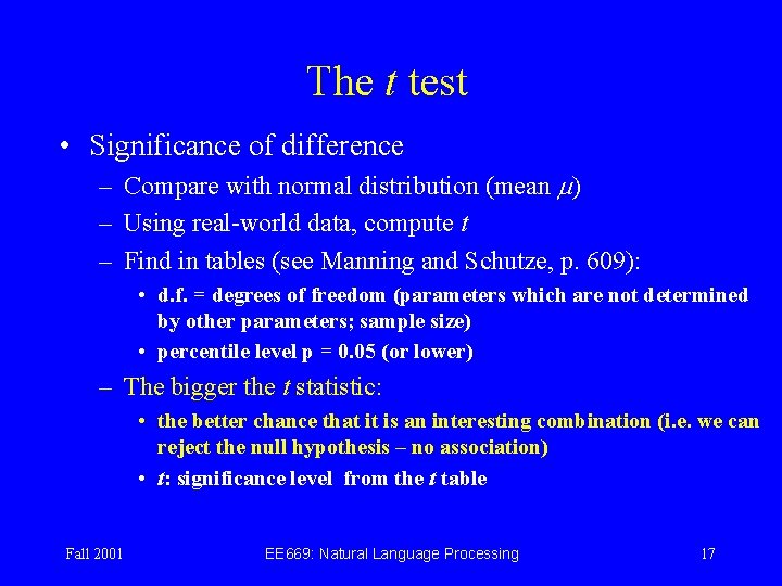
Hypothesis Testing: The t test • The t test looks at the mean and variance of a sample of measurements, where the null hypothesis is that the sample is drawn from a distribution with mean . • The test looks at the difference between the observed and expected means, scaled by the variance of the data, and tells us how likely one is to get a sample of that mean and variance assuming that the sample is drawn from a normal distribution with mean . Fall 2001 EE 669: Natural Language Processing 15

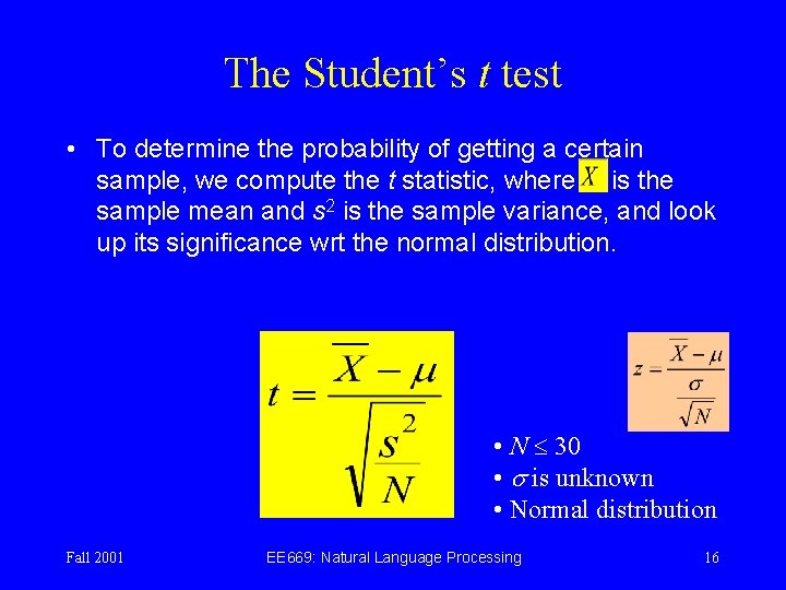
The Student’s t test • To determine the probability of getting a certain sample, we compute the t statistic, where is the sample mean and s 2 is the sample variance, and look up its significance wrt the normal distribution. • N 30 • is unknown • Normal distribution Fall 2001 EE 669: Natural Language Processing 16

The t test • Significance of difference – Compare with normal distribution (mean ) – Using real-world data, compute t – Find in tables (see Manning and Schutze, p. 609): • d. f. = degrees of freedom (parameters which are not determined by other parameters; sample size) • percentile level p = 0. 05 (or lower) – The bigger the t statistic: • the better chance that it is an interesting combination (i. e. we can reject the null hypothesis – no association) • t: significance level from the t table Fall 2001 EE 669: Natural Language Processing 17

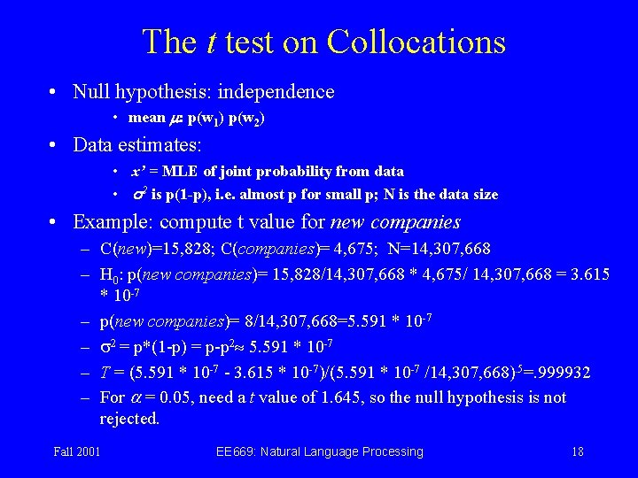
The t test on Collocations • Null hypothesis: independence • mean m: p(w 1) p(w 2) • Data estimates: • x’ = MLE of joint probability from data • s 2 is p(1 -p), i. e. almost p for small p; N is the data size • Example: compute t value for new companies – C(new)=15, 828; C(companies)= 4, 675; N=14, 307, 668 – H 0: p(new companies)= 15, 828/14, 307, 668 * 4, 675/ 14, 307, 668 = 3. 615 * 10 -7 – p(new companies)= 8/14, 307, 668=5. 591 * 10 -7 – s 2 = p*(1 -p) = p-p 2 5. 591 * 10 -7 – T = (5. 591 * 10 -7 - 3. 615 * 10 -7)/(5. 591 * 10 -7 /14, 307, 668). 5=. 999932 – For a = 0. 05, need a t value of 1. 645, so the null hypothesis is not rejected. Fall 2001 EE 669: Natural Language Processing 18

Hypothesis Testing of Differences (Church & Hanks, 1989) • We may also want to find words whose cooccurrence patterns best distinguish between two words (e. g. , strong versus powerful). This application can be useful for Lexicography. • The t test is extended to the comparison of the means under the assumption that they are normally distributed. • The null hypothesis is that the average difference is 0. Fall 2001 EE 669: Natural Language Processing 19

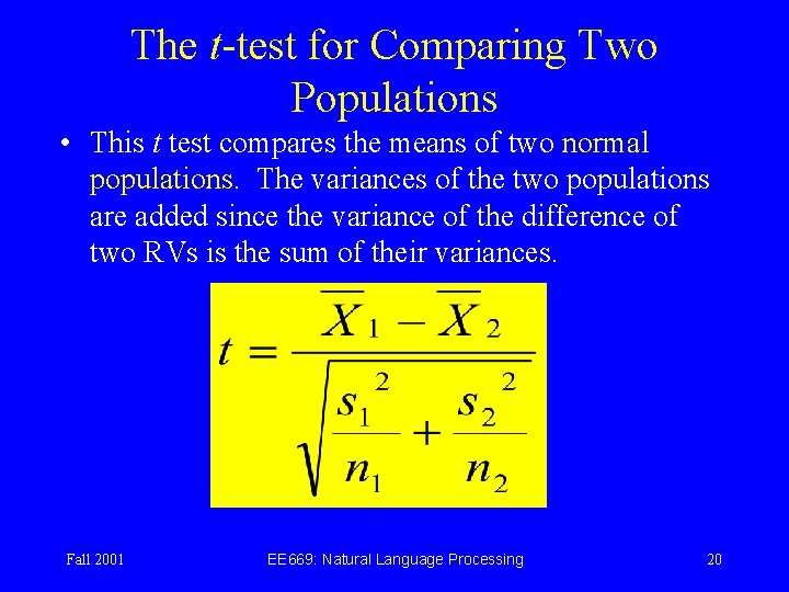
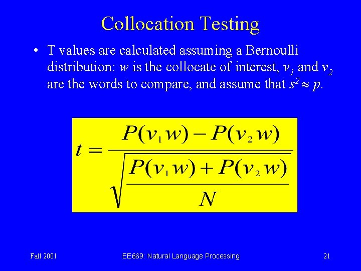
The t-test for Comparing Two Populations • This t test compares the means of two normal populations. The variances of the two populations are added since the variance of the difference of two RVs is the sum of their variances. Fall 2001 EE 669: Natural Language Processing 20

Collocation Testing • T values are calculated assuming a Bernoulli distribution: w is the collocate of interest, v 1 and v 2 are the words to compare, and assume that s 2 p. Fall 2001 EE 669: Natural Language Processing 21

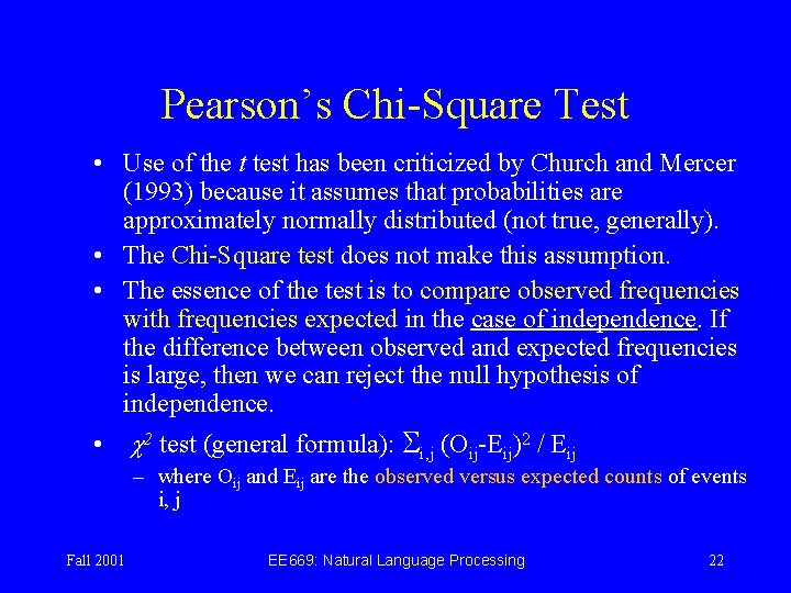
Pearson’s Chi-Square Test • Use of the t test has been criticized by Church and Mercer (1993) because it assumes that probabilities are approximately normally distributed (not true, generally). • The Chi-Square test does not make this assumption. • The essence of the test is to compare observed frequencies with frequencies expected in the case of independence. If the difference between observed and expected frequencies is large, then we can reject the null hypothesis of independence. • 2 test (general formula): Si, j (Oij-Eij)2 / Eij – where Oij and Eij are the observed versus expected counts of events i, j Fall 2001 EE 669: Natural Language Processing 22

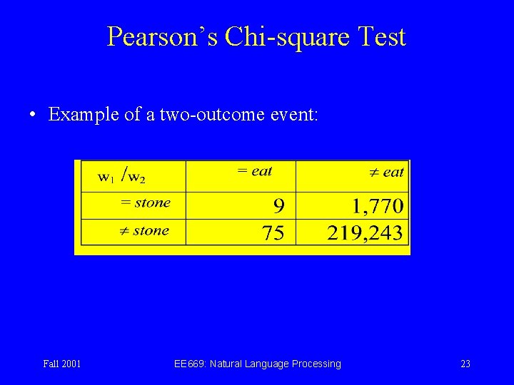
Pearson’s Chi-square Test • Example of a two-outcome event: Fall 2001 EE 669: Natural Language Processing 23

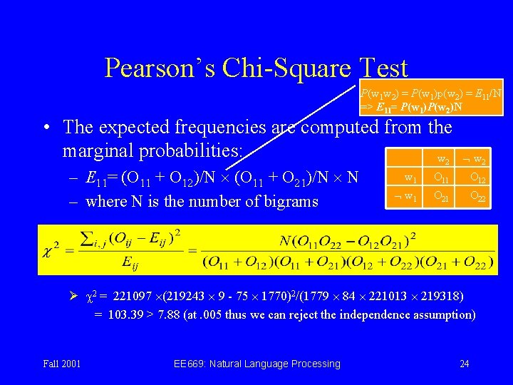
Pearson’s Chi-Square Test P(w 1 w 2) = P(w 1)p(w 2) = E 11/N => E 11= P(w 1)P(w 2)N • The expected frequencies are computed from the marginal probabilities: w – E 11= (O 11 + O 12)/N (O 11 + O 21)/N N – where N is the number of bigrams 2 w 2 w 1 O 12 w 1 O 22 Ø c 2 = 221097 (219243 9 - 75 1770)2/(1779 84 221013 219318) = 103. 39 > 7. 88 (at. 005 thus we can reject the independence assumption) Fall 2001 EE 669: Natural Language Processing 24

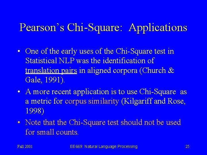
Pearson’s Chi-Square: Applications • One of the early uses of the Chi-Square test in Statistical NLP was the identification of translation pairs in aligned corpora (Church & Gale, 1991). • A more recent application is to use Chi-Square as a metric for corpus similarity (Kilgariff and Rose, 1998) • Note that the Chi-Square test should not be used for small counts. Fall 2001 EE 669: Natural Language Processing 25

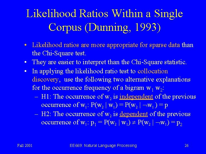
Likelihood Ratios Within a Single Corpus (Dunning, 1993) • Likelihood ratios are more appropriate for sparse data than the Chi-Square test. • They are easier to interpret than the Chi-Square statistic. • In applying the likelihood ratio test to collocation discovery, use the following two alternative explanations for the occurrence frequency of a bigram w 1 w 2: – H 1: The occurrence of w 2 is independent of the previous occurrence of w 1: P(w 2 | w 1) = P(w 2 | w 1 ) = p – H 2: The occurrence of w 2 is dependent of the previous occurrence of w 1: p 1 = P(w 2 | w 1) = p 2 Fall 2001 EE 669: Natural Language Processing 26

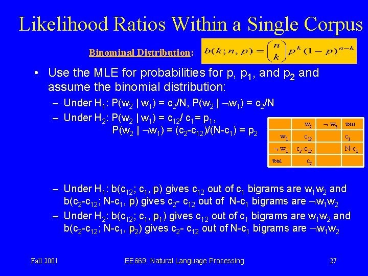
Likelihood Ratios Within a Single Corpus Binominal Distribution: • Use the MLE for probabilities for p, p 1, and p 2 and assume the binomial distribution: – Under H 1: P(w 2 | w 1) = c 2/N, P(w 2 | w 1) = c 2/N – Under H 2: P(w 2 | w 1) = c 12/ c 1= p 1, P(w 2 | w 1) = (c 2 -c 12)/(N-c 1) = p 2 w 1 c 12 w 1 c 2 -c 12 Total w 2 Total c 1 N-c 1 c 2 – Under H 1: b(c 12; c 1, p) gives c 12 out of c 1 bigrams are w 1 w 2 and b(c 2 -c 12; N-c 1, p) gives c 2 - c 12 out of N-c 1 bigrams are w 1 w 2 – Under H 2: b(c 12; c 1, p 1) gives c 12 out of c 1 bigrams are w 1 w 2 and b(c 2 -c 12; N-c 1, p 2) gives c 2 - c 12 out of N-c 1 bigrams are w 1 w 2 Fall 2001 EE 669: Natural Language Processing 27

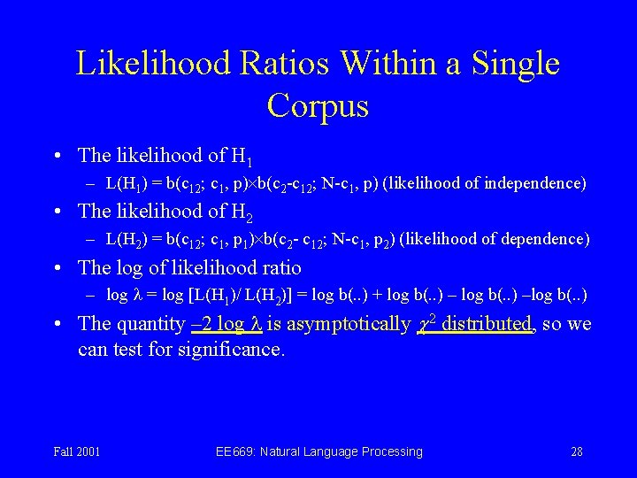
Likelihood Ratios Within a Single Corpus • The likelihood of H 1 – L(H 1) = b(c 12; c 1, p) b(c 2 -c 12; N-c 1, p) (likelihood of independence) • The likelihood of H 2 – L(H 2) = b(c 12; c 1, p 1) b(c 2 - c 12; N-c 1, p 2) (likelihood of dependence) • The log of likelihood ratio – log = log [L(H 1)/ L(H 2)] = log b(. . ) + log b(. . ) –log b(. . ) • The quantity – 2 log is asymptotically 2 distributed, so we can test for significance. Fall 2001 EE 669: Natural Language Processing 28

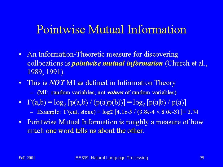
Pointwise Mutual Information • An Information-Theoretic measure for discovering collocations is pointwise mutual information (Church et al. , 1989, 1991). • This is NOT MI as defined in Information Theory – (MI: random variables; not values of random variables) • I’(a, b) = log 2 [p(a, b) / (p(a)p(b))] = log 2 [p(a|b) / p(a)] – Example: I’(eat, stone) = log 2 [4. 1 e-5 / (3. 8 e-4 8. 0 e-3) ]= 3. 74 • Pointwise Mutual Information is roughly a measure of how much one word tells us about the other. Fall 2001 EE 669: Natural Language Processing 29

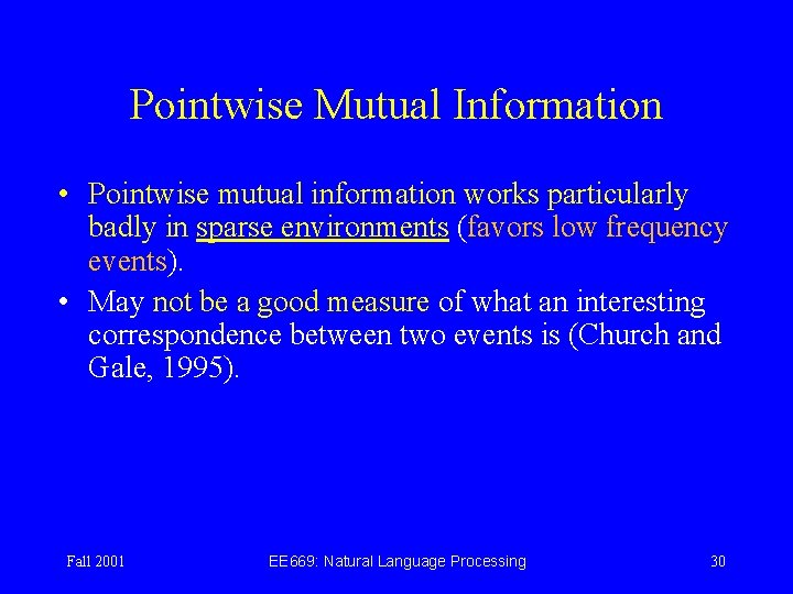
Pointwise Mutual Information • Pointwise mutual information works particularly badly in sparse environments (favors low frequency events). • May not be a good measure of what an interesting correspondence between two events is (Church and Gale, 1995). Fall 2001 EE 669: Natural Language Processing 30

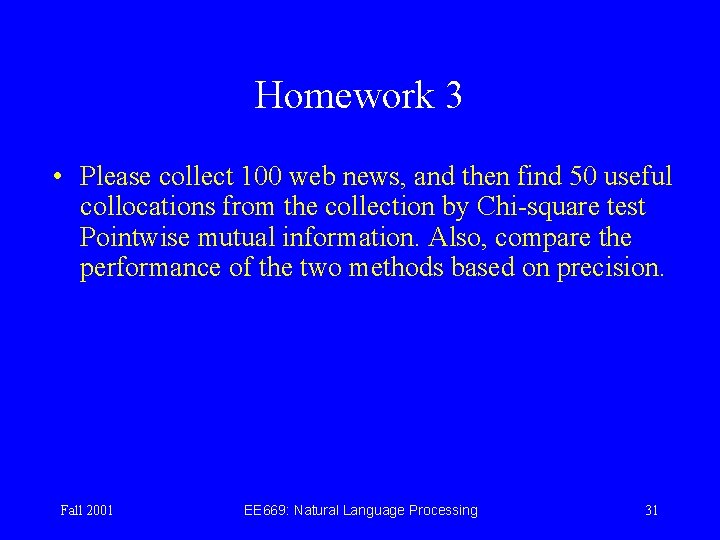
Homework 3 • Please collect 100 web news, and then find 50 useful collocations from the collection by Chi-square test Pointwise mutual information. Also, compare the performance of the two methods based on precision. Fall 2001 EE 669: Natural Language Processing 31