Lecture 5 Agenda Basic Contingency Table Analysis Rx

Lecture 5

Agenda • Basic Contingency Table Analysis – Rx. C Contingency Tables • Pearson Chi square test of association – Stratified 2 x 2 tables • Cochran Mantel Haenszel test of association • Breslow Day test of interaction • Simple Logistic Regression – Modeling dichotomous outcomes – Odds Ratios and Logistic Regression

Western Collaborative Group Study (WCGS) • Large scale prospective cohort study designed to examine risk factors for cardiovascular disease. • Main outcome is coronary heart disease (chd 69) – 1 = yes, 0 = no • Primary risk factor is personality type (dibpat) – 1 = type A, 0 = type B • Other risk factors collected as well: – Blood pressure, cholesterol, smoking, age, arcus senilis

Contingency table analysis • Historical precursor to logistic regression models. • What variables are associated with coronary heart disease? • Examples: – Arcus senilis (1 = present, 0 = not present) – Cholesterol (1 = < 200, 2 = 200 to 240, 3 = > 240) – Smoking (1 = 0 cigarettes/day, 2 = 1 -10, 3= 11 -20, 4= > 20)

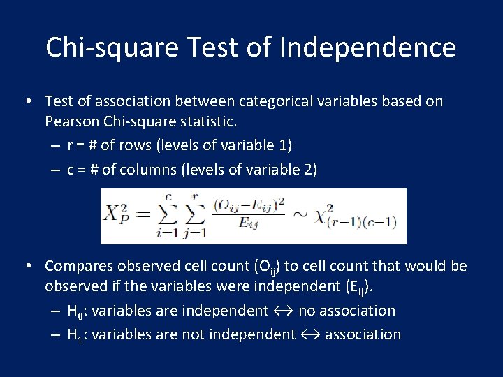
Chi-square Test of Independence • Test of association between categorical variables based on Pearson Chi-square statistic. – r = # of rows (levels of variable 1) – c = # of columns (levels of variable 2) • Compares observed cell count (Oij) to cell count that would be observed if the variables were independent (Eij). – H 0: variables are independent ↔ no association – H 1: variables are not independent ↔ association

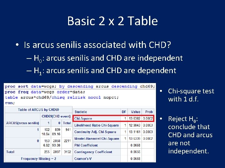
Basic 2 x 2 Table • Is arcus senilis associated with CHD? – H 0: arcus senilis and CHD are independent – H 1: arcus senilis and CHD are dependent • Chi-square test with 1 d. f. • Reject H 0: conclude that CHD and arcus are not independent.

Example: 2 x 2 Table • Use relrisk option in proc freq for this table. • Odds ratio interpretation – Odds of CHD are 1. 63 times higher for those with presence of arcus senilis compared to those without presence. • Relative risk interpretation – Risk (probability) of CHD is 1. 56 times higher for those with presence of arcus senilis compared to those without presence.

Stratified 2 x 2 Table • Arcus senilis is a condition associated with fatty deposits in the eye. • Also caused by widening of the eye vessels with age which makes it easier for fat to deposit. • May be of interest, therefore, to control for cholesterol and age. • Stratification allows us to divide a 2 x 2 table with respect to a third (and possibly 4 th variable).

Stratified 2 x 2 Table • Below we stratify by cholesterol group – Chol < 200, 200 <= chol < 240, chol > 240 • The Cochran Mantel Haenszel test allows us to compute the OR and RR adjusting for the stratifying variable (cholesterol group). • Use proc freq with cmh option to calculate the adjusted analysis statistics.

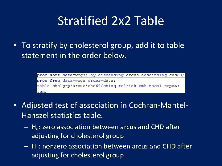
Stratified 2 x 2 Table • To stratify by cholesterol group, add it to table statement in the order below. • Adjusted test of association in Cochran-Mantel. Hanszel statistics table. – H 0: zero association between arcus and CHD after adjusting for cholesterol group – H 1: nonzero association between arcus and CHD after adjusting for cholesterol group

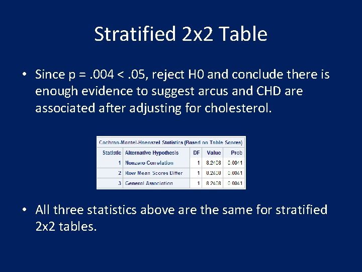
Stratified 2 x 2 Table • Since p =. 004 <. 05, reject H 0 and conclude there is enough evidence to suggest arcus and CHD are associated after adjusting for cholesterol. • All three statistics above are the same for stratified 2 x 2 tables.

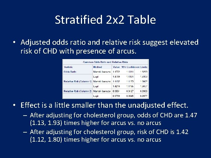
Stratified 2 x 2 Table • Adjusted odds ratio and relative risk suggest elevated risk of CHD with presence of arcus. • Effect is a little smaller than the unadjusted effect. – After adjusting for cholesterol group, odds of CHD are 1. 47 (1. 13, 1. 93) times higher for arcus vs. no arcus – After adjusting for cholesterol group, risk of CHD is 1. 42 (1. 12, 1. 80) times higher for arcus vs. no arcus

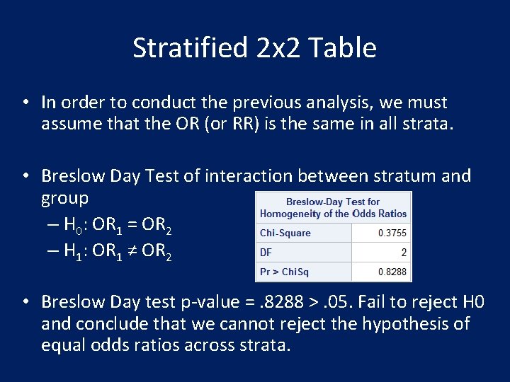
Stratified 2 x 2 Table • In order to conduct the previous analysis, we must assume that the OR (or RR) is the same in all strata. • Breslow Day Test of interaction between stratum and group – H 0: OR 1 = OR 2 – H 1: OR 1 ≠ OR 2 • Breslow Day test p-value =. 8288 >. 05. Fail to reject H 0 and conclude that we cannot reject the hypothesis of equal odds ratios across strata.

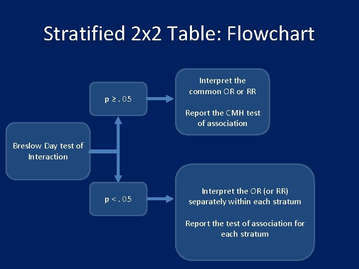
Stratified 2 x 2 Table: Flowchart p ≥. 05 Interpret the common OR or RR Report the CMH test of association Breslow Day test of Interaction p <. 05 Interpret the OR (or RR) separately within each stratum Report the test of association for each stratum

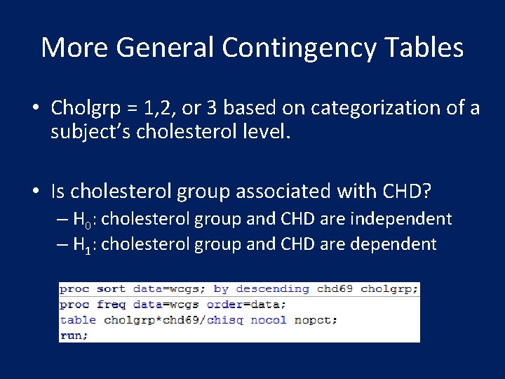
More General Contingency Tables • Cholgrp = 1, 2, or 3 based on categorization of a subject’s cholesterol level. • Is cholesterol group associated with CHD? – H 0: cholesterol group and CHD are independent – H 1: cholesterol group and CHD are dependent

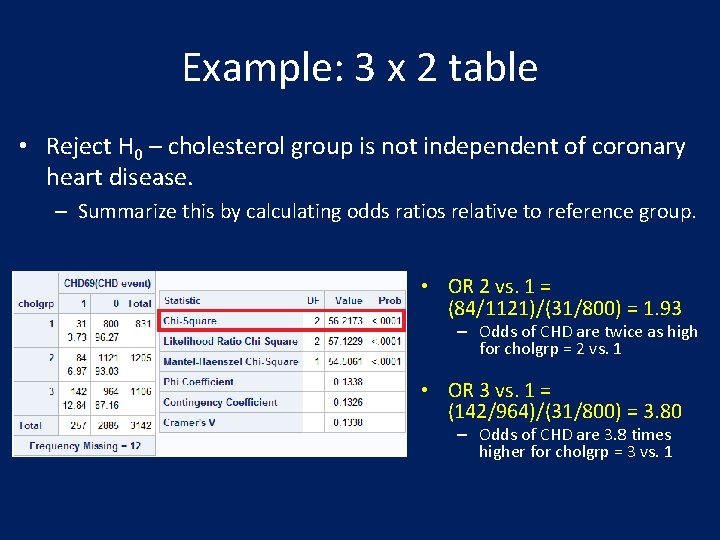
Example: 3 x 2 table • Reject H 0 – cholesterol group is not independent of coronary heart disease. – Summarize this by calculating odds ratios relative to reference group. • OR 2 vs. 1 = (84/1121)/(31/800) = 1. 93 – Odds of CHD are twice as high for cholgrp = 2 vs. 1 • OR 3 vs. 1 = (142/964)/(31/800) = 3. 80 – Odds of CHD are 3. 8 times higher for cholgrp = 3 vs. 1

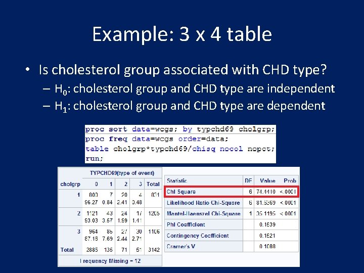
Example: 3 x 4 table • Is cholesterol group associated with CHD type? – H 0: cholesterol group and CHD type are independent – H 1: cholesterol group and CHD type are dependent

Contingency Table Analysis • Contingency table analysis is useful for descriptive purposes. • Some limitations – As dimensions increase it becomes harder to summarize the direction of association – Cannot estimate association of categorical and continuous variables (must categorize) – Multivariable modeling beyond one or two stratifying variables is cumbersome

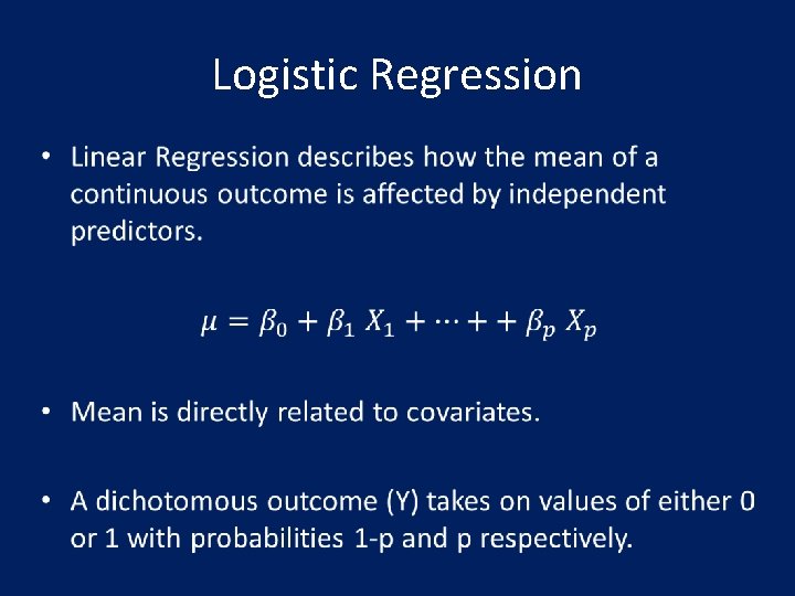
Logistic Regression •

Logistic Regression • Mean of a dichotomous outcome is equal to the probability of a “positive” outcome: p = P(Y=1). μ = 1*p + 0*(1 -p) = p • Cannot use linear regression. – 0 ≤ p ≤ 1 – Linear regression may estimate p > 1 or p < 0 since there is no constraint

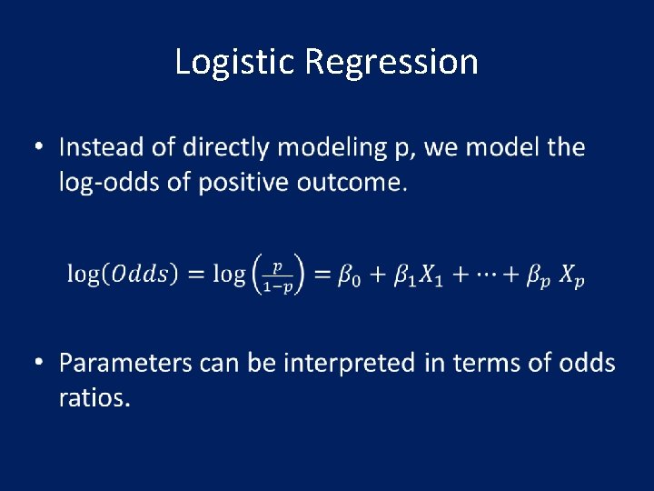
Logistic Regression •

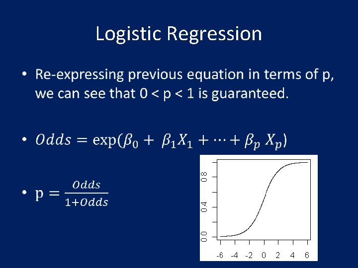
Logistic Regression •

Logistic Regression • βj is the adjusted log-odds ratio comparing unit differences in xj

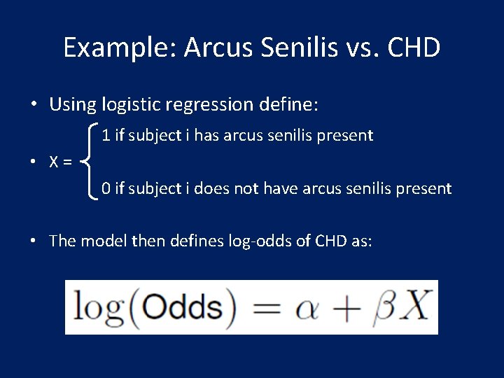
Example: Arcus Senilis vs. CHD • Using logistic regression define: 1 if subject i has arcus senilis present • X = 0 if subject i does not have arcus senilis present • The model then defines log-odds of CHD as:

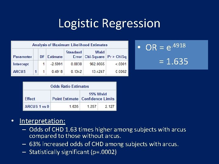
Logistic Regression • OR = e. 4918 = 1. 635 • Interpretation: – Odds of CHD 1. 63 times higher among subjects with arcus compared to those without arcus. – 63% increased odds of CHD among subjects with arcus. – Statistically significant (p=. 0002)

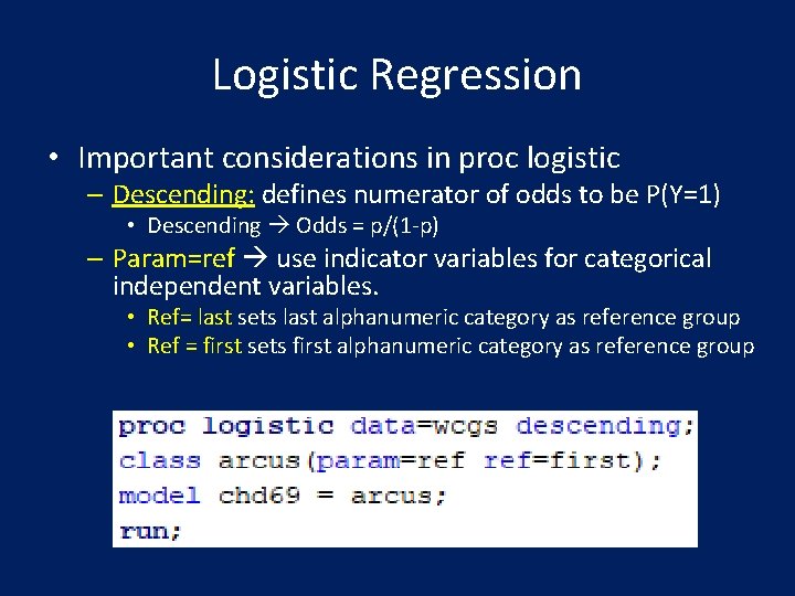
Logistic Regression • Important considerations in proc logistic – Descending: defines numerator of odds to be P(Y=1) • Descending Odds = p/(1 -p) – Param=ref use indicator variables for categorical independent variables. • Ref= last sets last alphanumeric category as reference group • Ref = first sets first alphanumeric category as reference group

Logistic Regression • Polychotomous Predictors – Pick a baseline (reference) group – Set up a series of indicators for all other groups – Should have k-1 Odds ratios comparing each group to baseline group. • Continuous Predictors – Compute Odds for two levels that differ by 1 -unit, odds ratio is then the exponentiated coefficient for the predictor. – Odds Ratio comparing c-unit differences in the predictor is ORc where OR is the 1 -unit odds ratio. – Confidence interval for c-unit OR comparisons are 1 -unit endpoints raised to the cth power.

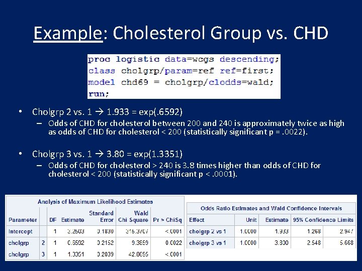
Example: Cholesterol Group vs. CHD • Cholgrp 2 vs. 1 1. 933 = exp(. 6592) – Odds of CHD for cholesterol between 200 and 240 is approximately twice as high as odds of CHD for cholesterol < 200 (statistically significant p =. 0022). • Cholgrp 3 vs. 1 3. 80 = exp(1. 3351) – Odds of CHD for cholesterol > 240 is 3. 8 times higher than odds of CHD for cholesterol < 200 (statistically significant p <. 0001).

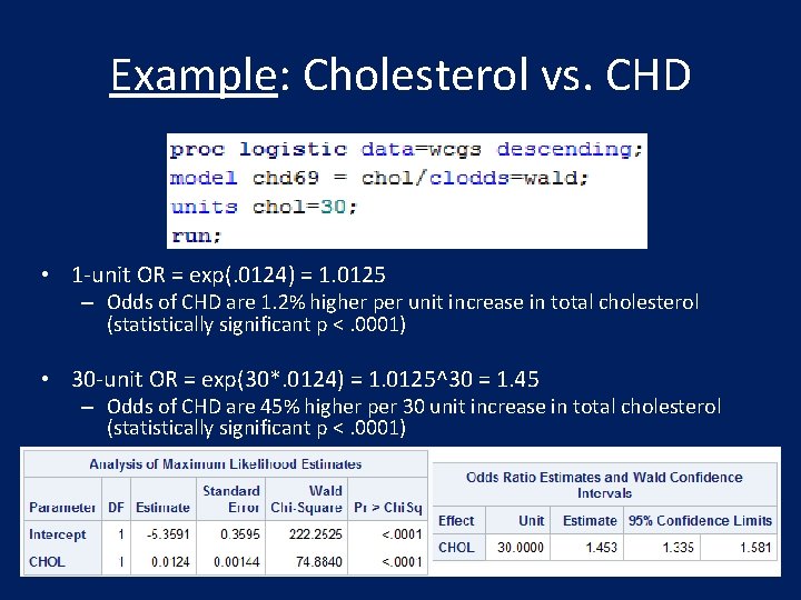
Example: Cholesterol vs. CHD • 1 -unit OR = exp(. 0124) = 1. 0125 – Odds of CHD are 1. 2% higher per unit increase in total cholesterol (statistically significant p <. 0001) • 30 -unit OR = exp(30*. 0124) = 1. 0125^30 = 1. 45 – Odds of CHD are 45% higher per 30 unit increase in total cholesterol (statistically significant p <. 0001)

Multivariable Logistic Regression • Basic principles of covariate adjustment and effect modification from linear regression carry over to logistic regression. • Use additional covariates to: – Control for potential confounders, other covariates – Build a stronger predictive model for the outcome – Describe effect modification (interaction)

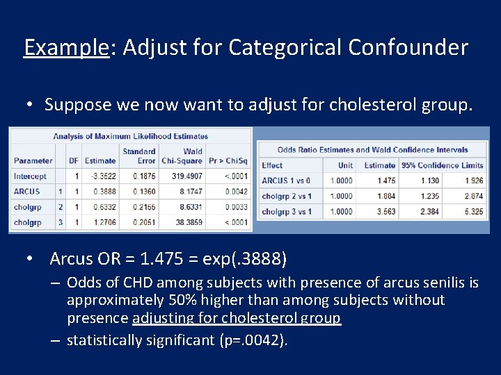
Example: Adjust for Categorical Confounder • Suppose we now want to adjust for cholesterol group. • Arcus OR = 1. 475 = exp(. 3888) – Odds of CHD among subjects with presence of arcus senilis is approximately 50% higher than among subjects without presence adjusting for cholesterol group – statistically significant (p=. 0042).

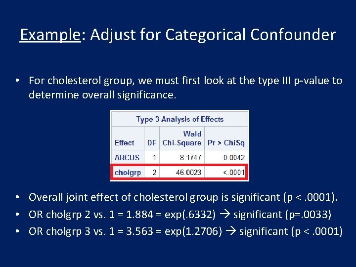
Example: Adjust for Categorical Confounder • For cholesterol group, we must first look at the type III p-value to determine overall significance. • Overall joint effect of cholesterol group is significant (p <. 0001). • OR cholgrp 2 vs. 1 = 1. 884 = exp(. 6332) significant (p=. 0033) • OR cholgrp 3 vs. 1 = 3. 563 = exp(1. 2706) significant (p <. 0001)

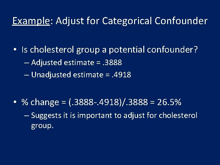
Example: Adjust for Categorical Confounder • Is cholesterol group a potential confounder? – Adjusted estimate =. 3888 – Unadjusted estimate =. 4918 • % change = (. 3888 -. 4918)/. 3888 = 26. 5% – Suggests it is important to adjust for cholesterol group.

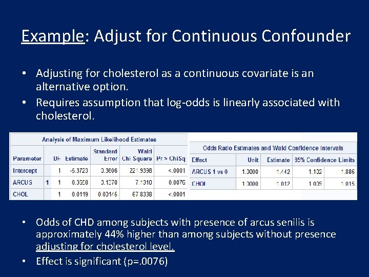
Example: Adjust for Continuous Confounder • Adjusting for cholesterol as a continuous covariate is an alternative option. • Requires assumption that log-odds is linearly associated with cholesterol. • Odds of CHD among subjects with presence of arcus senilis is approximately 44% higher than among subjects without presence adjusting for cholesterol level. • Effect is significant (p=. 0076)

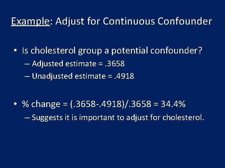
Example: Adjust for Continuous Confounder • Is cholesterol group a potential confounder? – Adjusted estimate =. 3658 – Unadjusted estimate =. 4918 • % change = (. 3658 -. 4918)/. 3658 = 34. 4% – Suggests it is important to adjust for cholesterol.

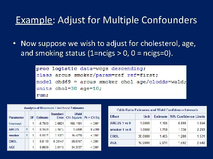
Example: Adjust for Multiple Confounders • Now suppose we wish to adjust for cholesterol, age, and smoking status (1=ncigs > 0, 0 = ncigs=0).

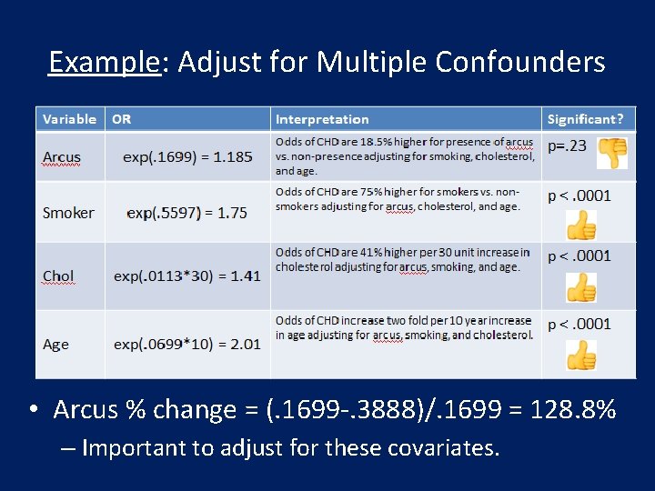
Example: Adjust for Multiple Confounders • Arcus % change = (. 1699 -. 3888)/. 1699 = 128. 8% – Important to adjust for these covariates.