Lecture 5 6 xxxxxxx 5 3 More Realistic

Lecture 5 -6 xxxxxxx

5. 3 More Realistic Nuclear Models q Both the shell model for odd-A nuclei and the collective model for even nuclei are idealizations that are only approximately valid for real nuclei, which are far more complex in their structure than our simple models suggest. q Moreover, in real nuclei we cannot “ turn off” one type of structure and consider only the other. q Thus even very collective nuclei show single-particle effects, while the q core of nucleons in shell-model nuclei may contribute collective effects that we have ignored up to this point. q The structure of most nuclei cannot be quite so neatly divided between single-particle and collective motion, and usually we must consider a combination of both. q Such a unified nuclear model is mathematically too complicated to be discussed here, and hence we will merely illustrate a few of the resulting properties of nuclei and try to relate them to the more elementary aspects of the shell and collective models. q Many-Particle Shell Model q In our study of the shell model, we considered only the effects due to the last unpaired single particle. q A more realistic approach for odd-A nuclei would be to include all particles outside of closed shells. q Let us consider for example the nuclei with odd 2 or N between 20 and

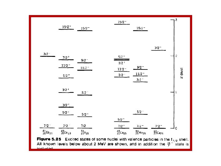
q The nuclei whose structure is determined by a single particle (41 Ca and 55 C 0) show the expected levels-a f - ground state, corresponding to the single odd f 7/2 particle (or vacancy, in the case of 55 C 0, since a single vacancy or hole in a shell behaves like a single particle in the shell), and a +- excited state at about 2 Me. V, corresponding to exciting the single odd particle to the p 3/2 state. q The nuclei with 3 or 5 particles in the f 7/2 level show a much richer spectrum of states, and in particular the very low negative-parity states cannot be explained by the extreme single-particle shell model. q If the ; - state, for instance, originated from the excitation of a single particle to the f 5/2 shell, we would expect it to appear above 2 Me. V because the f 5/2 level occurs above the p 3/2 level (see Figure 5. 6); the lowest 2 - level in the single-particle nuclei occurs at 2. 6 Me. V (in 41 Ca) and 3. 3 Me. V (in 55 C 0). q We use the shorthand notation (f 7/!)n to indicate the configuration with n particles in the f 7/2 shell, and we consider the possible resultant values of I for the configuration (f 712)~. q (From the symmetry between particles and holes, the levels of three holes, or five particles, in the f 7, 2 shell will be the same. ) q Because the nucleons have half-integral spins, they must obey the Pauli principle, and thus no two particles can have the same set of quantum numbers. q Each particle in the shell model is described by the angular momentum j = : , which can have the projections or z components corresponding to m = &

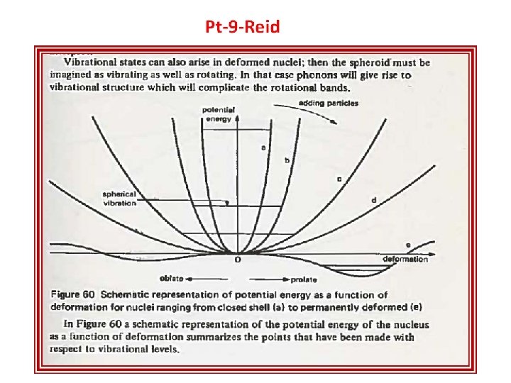
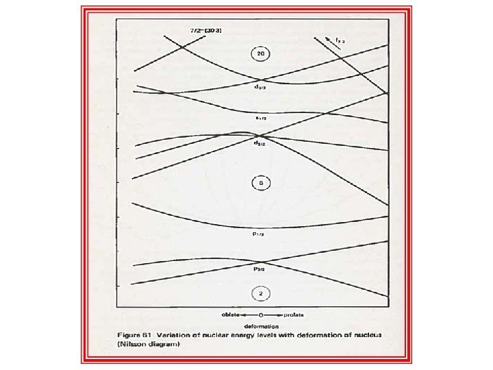
q Single-Particle States in Deformed Nuclei q The calculated levels of the nuclear shell model are based on the assumption that the nuclear potential is spherical. q We know, however, that this is not true for nuclei in the range 150 I A I 19 0 and A > 230. q For these nuclei we should use a shell-model potential that approximates the actual nuclear shape, specifically a rotational ellipsoid. q In calculations using the Schrodinger equation with a nonspherical potential, the angular momentum e is no longer a “good” quantum number; that is, we cannot identify states by their spectroscopic notation (s, p, d, f, etc. ) as we did for the spherical shell model. q To put it another way, the states that result from the calculation have mixtures of different 8 values (but based on consideration of parity, we expect mixtures of only even or only odd t values). q In the spherical case, the energy levels of each single particle state have a degeneracy of (2 j + 1). q (That is, relative to any arbitrary axis of our choice, all 2 j + 1 possible orientations of j are equivalent. ) q If the potential has a deformed shape, this will no longer be true-the energy levels in the deformed potential depend on the spatial orientation of the orbit. q More precisely, the energy depends on the component of j along the symmetry axis of the core. q For example, an f 7, 2 nucleon can have eight possible components of j ,

q The Pauli principle requires that each of the 3 particles have a different value of m. q Immediately we conclude that the maximum value of the total projection, q M = m, + m 2+ m 3, fo r the three particles is + $ + = + y. q ( Without the Pauli principle, the maximum would be y. ) q We therefore expect to find no state in the configuration (f, , 2)3 with I greater than y; the maximum resultant angular momentum is I = y, which can have all possible M from + Y to - Y. q The next highest possible M is y, which can only be obtained from + 3 + + q (+ 5 + 1 + state must belong to the M states we have already assigned to the I = configuration; thus we have no possibility to have a I = resultant. Continuing in this way, we find two possibilities to obtain M = + (+: + 2 + $ and + f - + + $); there are thus two possible M = + configuration and another that we can assign to I = y. q Extending this reasoning, we expect to find the following states for (f 7, 2)3 or (f 7, f)5: I = y, y, z, ; , $, and t. q Because each of the three or five particles has negative parity, the resultant parity is (--l)3 T. h e nuclei shown in Figure 5. 25 show low-lying negative-parity states with the expected spins (and also with the expected absences-no low-lying : - or y - states appear). q +is not permitted, nor is + ; + - $). q This single M = states, one for the I = q Although this analysis is reasonably successful, it is incomplete-if we do q indeed treat all valence particles as independent and equivalent, then the

This is obviously not even approximately true; in the case of the (f 7, 2)3 multiplet, the energy splitting between the highest and lowest energy levels is 2. 7 Me. V, about the same energy as pair-breaking and particle-exciting interactions. We can analyze these energy splittings in terms of a residual interaction between the valence particles, and thus the level structure of these nuclei gives us in effect a way to probe the nucleon interaction in an environment different from the free-nucleon studies we discussed in Chapter 4. As a final comment, we state without proof that the configurations with n particles in the same shell have another common feature that lends itself to experimental test- their magnetic moments should all be proportional to I. That is, given two different states 1 and 2 belonging to the same configuration, we expect l. U 1 -- -I 1 P 2 I 2 (5. 21) Unfortunately, few of the excited-state magnetic moments are well enough known to test this prediction. In the case of 51 V, the ground-state moment is p = +5. 1514 f 0. 0001 p. N and the moment of the first excited state is p = +3. 86 & 0. 33 p. N. The ratio of the moments is thus 1. 33 f 0. 11, in agreement with the expected ratio : / 2 = 1. 4. In the case of 53 Mn, the ratio of moments of the same states is 5. 024 f

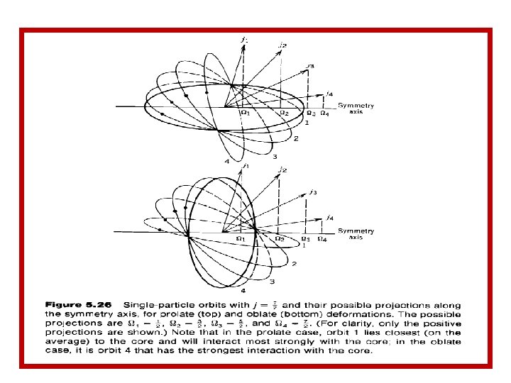
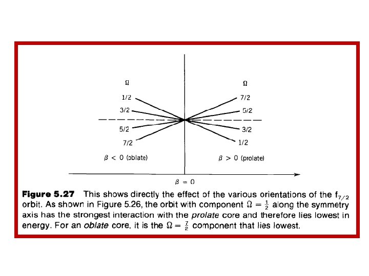
This component of j along the symmetry axis is generally denoted by 8. Because the nuclei have reflection symmetry for either of the two possible directions of the symmetry axis, the components +8 and -8 will have the same energy, giving the levels a degeneracy of 2. That is, what we previously called the f 7/2 state splits up into four states if we deform the central potential; these states are labeled 8 = +, t, $, and all have negative parity. Figure 5. 26 indicates the different possible “orbits” of the odd particle for prolate and oblate deformations. For prolate deformations, the orbit with the smallest possible 8 (equal to i) interacts most strongly with the core and is thus more tightly bound and lowest in energy. The situation is different for oblate deformations, in which the orbit with maximum 8 (equal to j ) has the strongest interaction with the core and the lowest energy. Figure 5. 27 shows how the f 7/2 states would split as the deformation is increased. Of course, we must keep in mind that Figures 5. 26 and 5. 27 are not strictly correct because the spherical single-particle quantum numbers t and j are not valid when the potential is deformed. The negative parity state with 8 = : , for example, cannot be identified with the f 7/2 state, even though it approaches that state as p + 0. The wave function of the 8 = 5 state can be expressed as a mixture (or linear combination) of many different t and j (but only with j 2 5,

It is customary to make the approximation that states from different major oscillator shells (see Figures 5. 4 and 5. 6) do not mix. Thus, for example, the 8 = 1 state that approaches the 2 f 7/, level as p --+ 0 will include contributions from only those states of the 5 th oscillator shell (2 f 5, , , 2 f 7, , , 1 hg. I 2, lhll 12). The 4 th and 6 th oscillator shells have the opposite parity and so will not mix, and the next odd-parity shells are far away and do not mix strongly. Writing the spherical wave functions as GNej, we must have (5. 22) where +'(8) represents the wave function of the deformed state 8 and where a(NL'j) are the expansion coefficients. For the 8 = : state The coefficients a( N t j ) can be obtained by solving the Schrodinger equation for the deformed potential, which was first done by S. G. Nilsson in 1955. The coefficients will vary with p, and of course for p + 0 we expect ~ ( 5 3 : ) to approach 1 while the others all approach 0. For , 8 = 0. 3 (a typical prolate deformation), Nilsson calculated the values ~ ( 5 3 ; )= 0. 267 ~ ( 5 5 : ) = 0. 415 a(53: ) = 0. 832 a(55 y) = -0. 255 for the 8 = 5 level we have been considering. Given such wave functions for single-particle states in deformed nuclei, we can then allow the nuclei to rotate, and we expect to find a sequence of

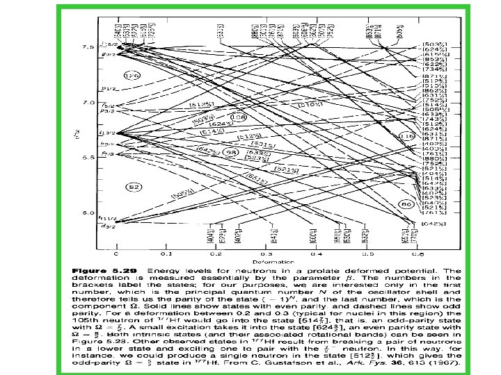
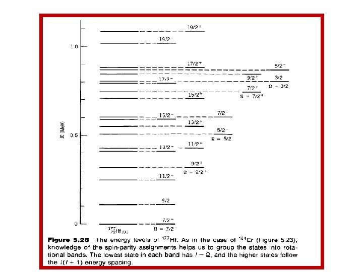
The lowest state of the rotational band has I = Q, and as rotational energy is added the angular momentum increases in the sequence I = $2, 52 + 1, Q + 2, . . Figure 5. 28 shows the energy levels of the nucleus 177 Hfi, n which two welldeveloped rotational bands have been found and several other single-particle states have been identified. To interpret the observed single-particle levels, we require a diagram similar to Figure 5. 27 but which shows all possible single-particle states and how their energies vary with deformation. Such a diagram is shown in Figure 5. 29 for the neutron states that are appropriate to the 150 I A I 190 region. Recalling that the degeneracy of each deformed single-particle level is 2, we proceed exactly as we did in the spherical shell model, placing two neutrons in each state up to N = 105 and two protons in each state up to 2 = 72. We can invoke the pairing argument to neglect the single-particle states of the protons and examine the possible levels of the 105 th neutron for the typical deformation of p = 0. 3. You can see from the diagram that the expected single-particle levels correspond exactly with the observed levels of 177 Hf. The general structure of the odd-A deformed nuclei is thus characterized by rotational bands built on single-particle states calculated from the deformed shell-model potential. The proton and neutron states are filled (two nucleons per state), and the nuclear properties are determined in the extreme single-particle

This model, with the wave functions calculated by Nilsson, has had extraordinary success in accounting for the nuclear properties in this region. In general, the calculations based on the properties of the odd particle have been far more successful in the deformed region than have the analogous calculations in the spherical region. In this chapter we have discussed evidence for types of nuclear structure based on the static properties of nuclei- energy levels, spin-parity assignments, magnetic dipole and electric quadrupole moments. The wave functions that result from solving the Schrodinger equation for these various models permit many other features of nuclear structure to be calculated, particularly the transitions between different nuclear states. Often the evidence for collective structure, for instance, may be inconclusive based on the energy levels alone, while the transition probabilities between the excited states may give definitive proof of collective effects. It may also be the case that a specific excited state may have alternative interpretations- for example, a vibrational state or a 2 -particle coupling. Studying the transition probabilities will usually help us to discriminate between these competing interpretations. The complete study of nuclear structure therefore requires that we study radioactive decays, which give spontaneous transitions between states, and nuclear reactions, in which the experimenter can select the initial and final states. In both cases, we can compare calculated decay and reaction probabilities with