Lecture 45 CHS 221 DR Wajed Hatamleh Slide

Lecture # 4&5 CHS 221 DR. Wajed Hatamleh Slide 1

Slide 2 variance i

Definition Slide 3 v The variance of a set of values is a measure of variation equal to the square of the standard deviation. v Sample variance: Square of the sample standard deviation s v Population variance: Square of the population standard deviation

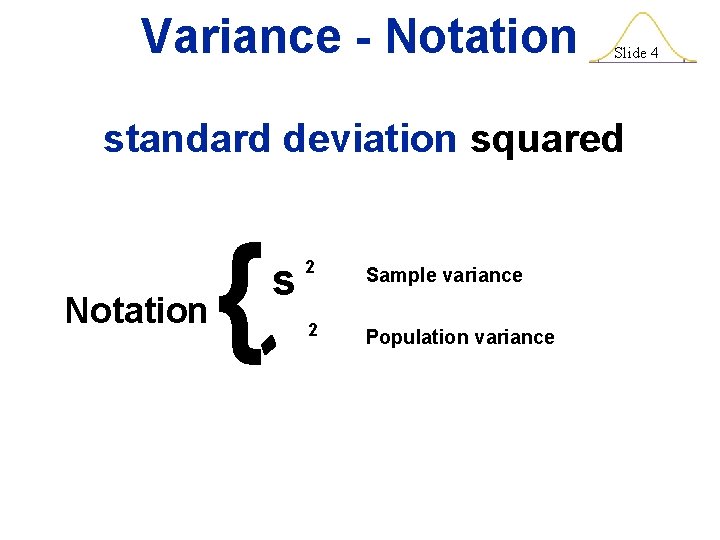
Variance - Notation Slide 4 standard deviation squared } Notation s 2 Sample variance 2 Population variance

Slide 5 Measures of Relative Standing ia

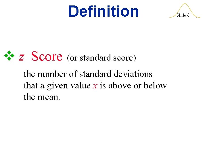
Definition v z Score (or standard score) the number of standard deviations that a given value x is above or below the mean. Slide 6

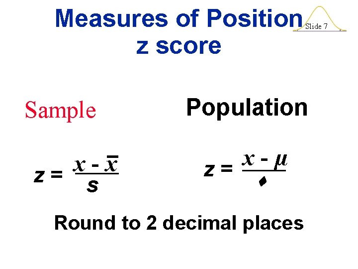
Measures of Position z score Sample x x z= s Slide 7 Population x µ z= Round to 2 decimal places

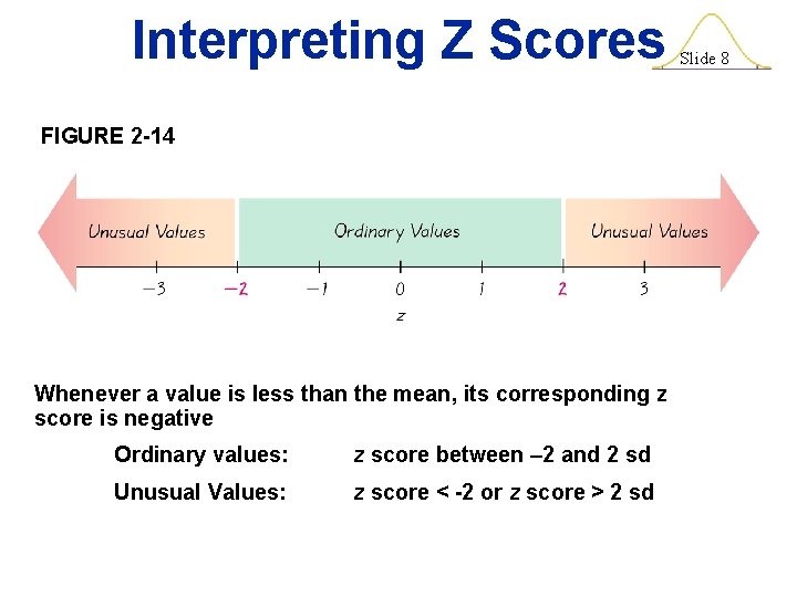
Interpreting Z Scores FIGURE 2 -14 Whenever a value is less than the mean, its corresponding z score is negative Ordinary values: z score between – 2 and 2 sd Unusual Values: z score < -2 or z score > 2 sd Slide 8

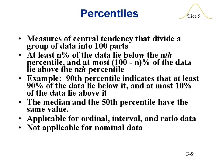
Percentiles Slide 9 • Measures of central tendency that divide a group of data into 100 parts • At least n% of the data lie below the nth percentile, and at most (100 - n)% of the data lie above the nth percentile • Example: 90 th percentile indicates that at least 90% of the data lie below it, and at most 10% of the data lie above it • The median and the 50 th percentile have the same value. • Applicable for ordinal, interval, and ratio data • Not applicable for nominal data 3 -9

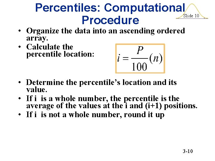
Percentiles: Computational. Slide 10 Procedure • Organize the data into an ascending ordered array. • Calculate the percentile location: • Determine the percentile’s location and its value. • If i is a whole number, the percentile is the average of the values at the i and (i+1) positions. • If i is not a whole number, round it up 3 -10

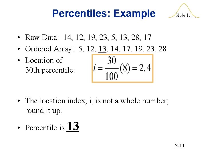
Percentiles: Example Slide 11 • Raw Data: 14, 12, 19, 23, 5, 13, 28, 17 • Ordered Array: 5, 12, 13, 14, 17, 19, 23, 28 • Location of 30 th percentile: • The location index, i, is not a whole number; round it up. • Percentile is 13 3 -11

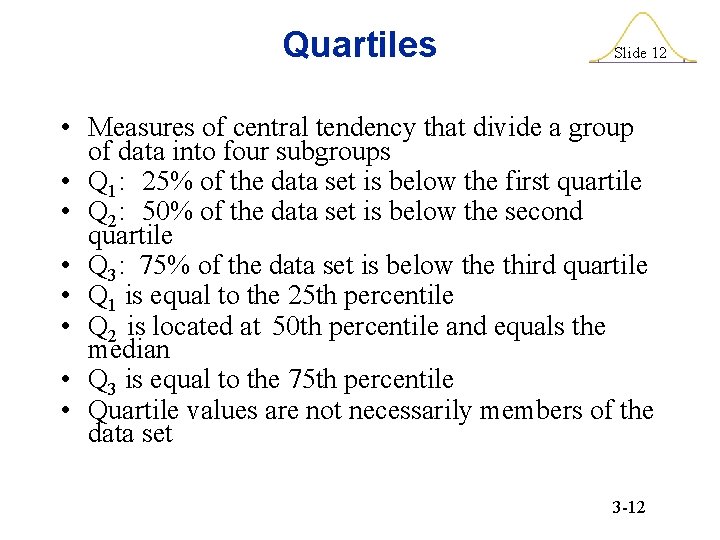
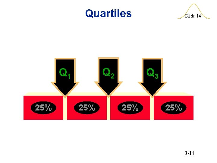
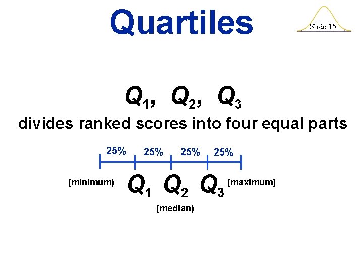
Quartiles Slide 12 • Measures of central tendency that divide a group of data into four subgroups • Q 1: 25% of the data set is below the first quartile • Q 2: 50% of the data set is below the second quartile • Q 3: 75% of the data set is below the third quartile • Q 1 is equal to the 25 th percentile • Q 2 is located at 50 th percentile and equals the median • Q 3 is equal to the 75 th percentile • Quartile values are not necessarily members of the data set 3 -12

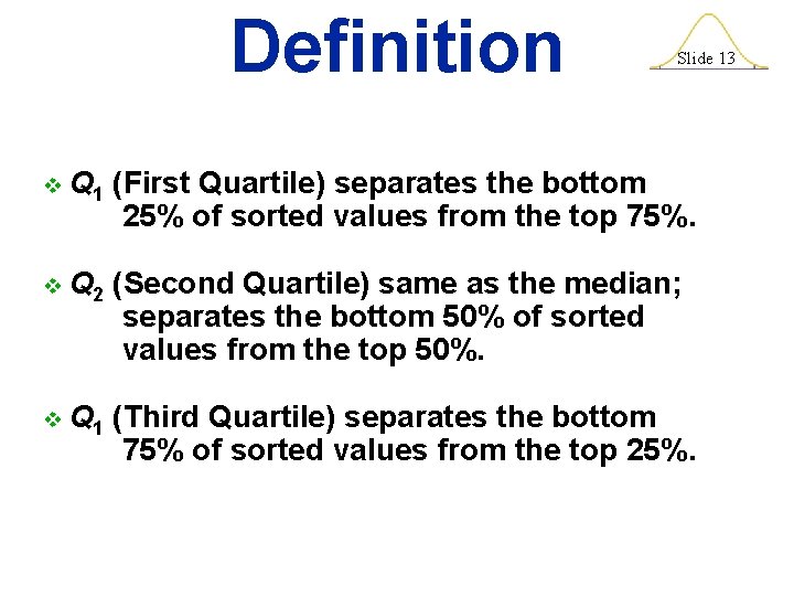
Definition Slide 13 v Q 1 (First Quartile) separates the bottom 25% of sorted values from the top 75%. v Q 2 (Second Quartile) same as the median; separates the bottom 50% of sorted values from the top 50%. v Q 1 (Third Quartile) separates the bottom 75% of sorted values from the top 25%.

Quartiles Q 2 Q 1 25% Slide 14 Q 3 25% 3 -14

Quartiles Slide 15 Q 1, Q 2, Q 3 divides ranked scores into four equal parts 25% (minimum) 25% 25% Q 1 Q 2 Q 3 (median) (maximum)

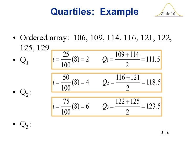
Quartiles: Example Slide 16 • Ordered array: 106, 109, 114, 116, 121, 122, 125, 129 • Q 1 • Q 2: • Q 3: 3 -16

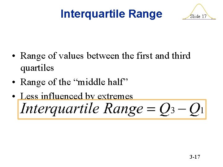
Interquartile Range Slide 17 • Range of values between the first and third quartiles • Range of the “middle half” • Less influenced by extremes 3 -17

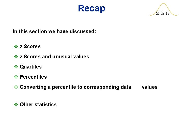
Recap Slide 18 In this section we have discussed: v z Scores and unusual values v Quartiles v Percentiles v Converting a percentile to corresponding data v Other statistics values

Slide 19 Exploratory Data Analysis (EDA)

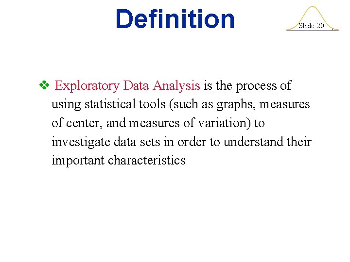
Definition Slide 20 v Exploratory Data Analysis is the process of using statistical tools (such as graphs, measures of center, and measures of variation) to investigate data sets in order to understand their important characteristics

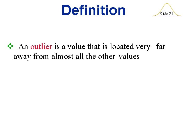
Definition Slide 21 v An outlier is a value that is located very far away from almost all the other values

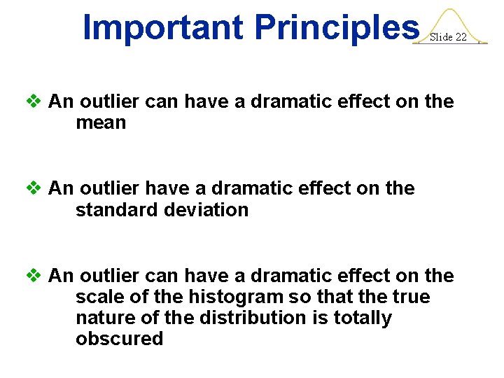
Important Principles Slide 22 v An outlier can have a dramatic effect on the mean v An outlier have a dramatic effect on the standard deviation v An outlier can have a dramatic effect on the scale of the histogram so that the true nature of the distribution is totally obscured

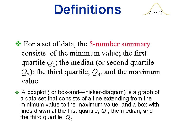
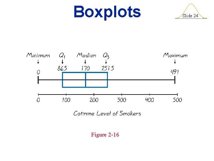
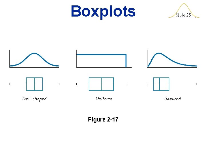
Definitions Slide 23 v For a set of data, the 5 -number summary consists of the minimum value; the first quartile Q 1; the median (or second quartile Q 2); the third quartile, Q 3; and the maximum value v A boxplot ( or box-and-whisker-diagram) is a graph of a data set that consists of a line extending from the minimum value to the maximum value, and a box with lines drawn at the first quartile, Q 1; the median; and the third quartile, Q 3

Boxplots Figure 2 -16 Slide 24

Boxplots Figure 2 -17 Slide 25

Recap In this section we have looked at: v Exploratory Data Analysis v Effects of outliers v 5 -number summary and boxplots Slide 26

Slide 27 Probability

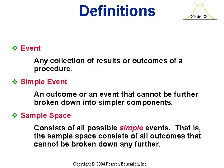
Definitions Slide 28 v Event Any collection of results or outcomes of a procedure. v Simple Event An outcome or an event that cannot be further broken down into simpler components. v Sample Space Consists of all possible simple events. That is, the sample space consists of all outcomes that cannot be broken down any further. Copyright © 2004 Pearson Education, Inc.

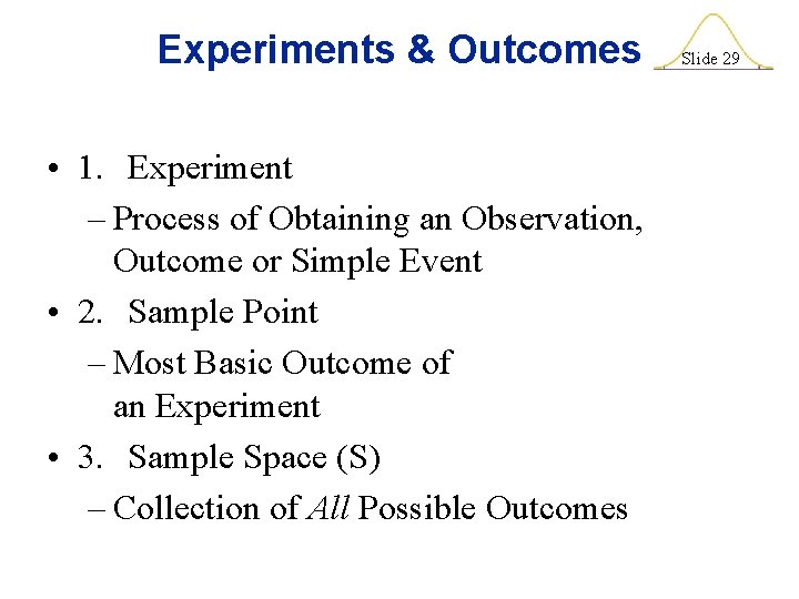
Experiments & Outcomes • 1. Experiment – Process of Obtaining an Observation, Outcome or Simple Event • 2. Sample Point – Most Basic Outcome of an Experiment • 3. Sample Space (S) – Collection of All Possible Outcomes Slide 29

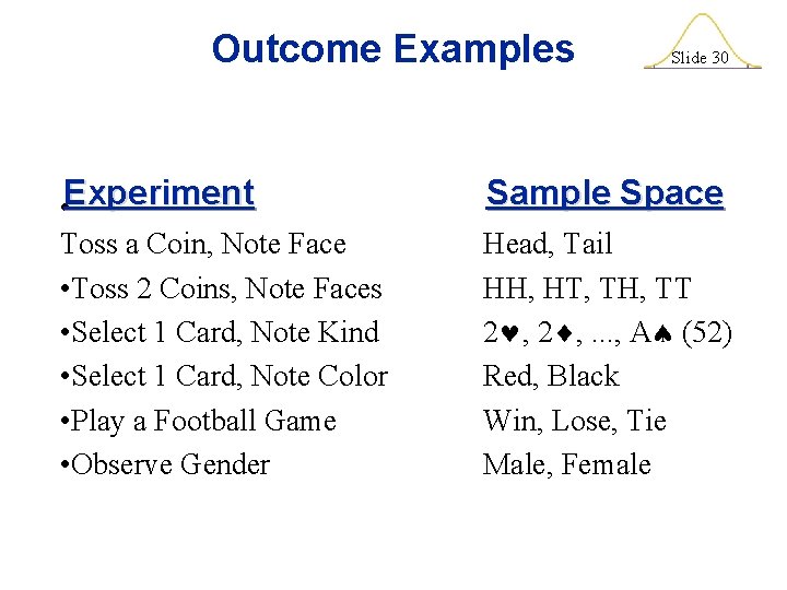
Outcome Examples • Experiment Toss a Coin, Note Face • Toss 2 Coins, Note Faces • Select 1 Card, Note Kind • Select 1 Card, Note Color • Play a Football Game • Observe Gender Slide 30 Sample Space Head, Tail HH, HT, TH, TT 2 , . . . , A (52) Red, Black Win, Lose, Tie Male, Female

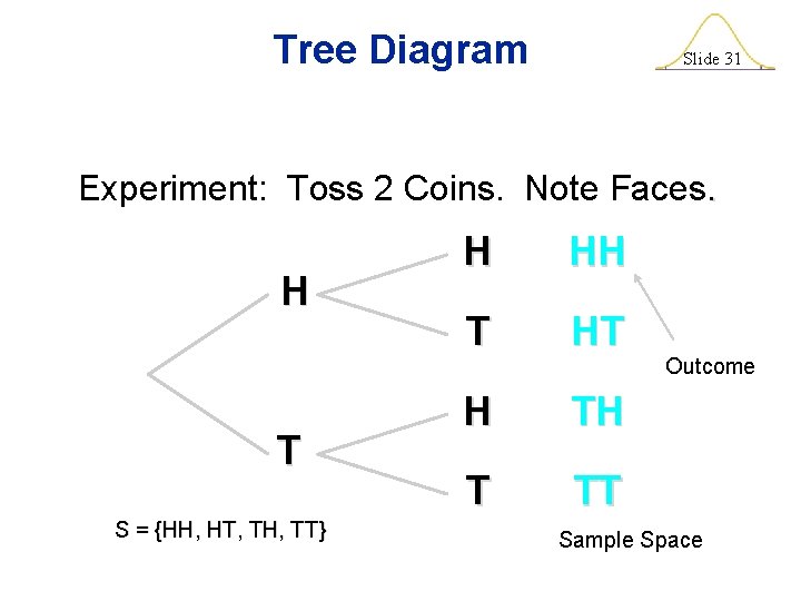
Tree Diagram Slide 31 Experiment: Toss 2 Coins. Note Faces. H T S = {HH, HT, TH, TT} H HH T HT H TH T TT Outcome Sample Space

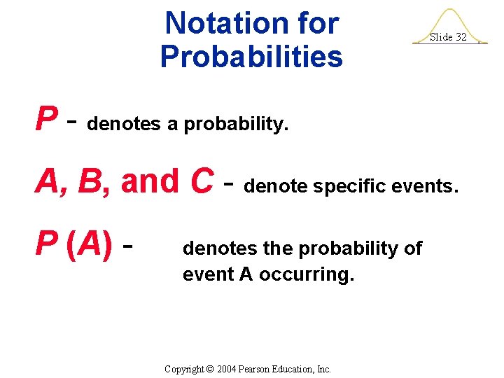
Notation for Probabilities Slide 32 P - denotes a probability. A, B, and C - denote specific events. P (A) - denotes the probability of event A occurring. Copyright © 2004 Pearson Education, Inc.

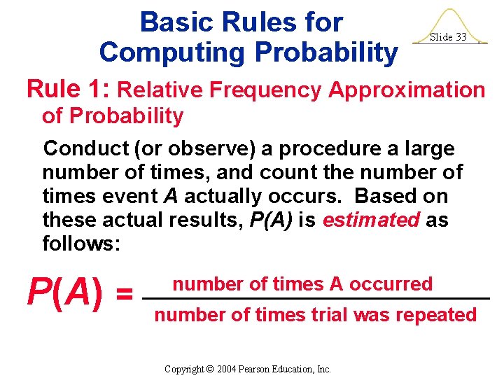
Basic Rules for Computing Probability Slide 33 Rule 1: Relative Frequency Approximation of Probability Conduct (or observe) a procedure a large number of times, and count the number of times event A actually occurs. Based on these actual results, P(A) is estimated as follows: P(A) = number of times A occurred number of times trial was repeated Copyright © 2004 Pearson Education, Inc.

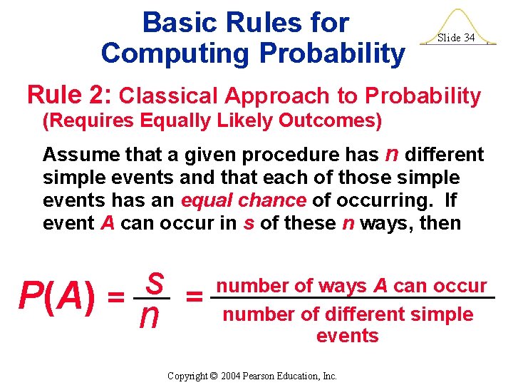
Basic Rules for Computing Probability Slide 34 Rule 2: Classical Approach to Probability (Requires Equally Likely Outcomes) Assume that a given procedure has n different simple events and that each of those simple events has an equal chance of occurring. If event A can occur in s of these n ways, then s = P(A) = n number of ways A can occur number of different simple events Copyright © 2004 Pearson Education, Inc.

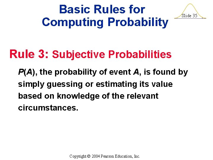
Basic Rules for Computing Probability Slide 35 Rule 3: Subjective Probabilities P(A), the probability of event A, is found by simply guessing or estimating its value based on knowledge of the relevant circumstances. Copyright © 2004 Pearson Education, Inc.

Law of Large Numbers Slide 36 As a procedure is repeated again and again, the relative frequency probability (from Rule 1) of an event tends to approach the actual probability. Copyright © 2004 Pearson Education, Inc.

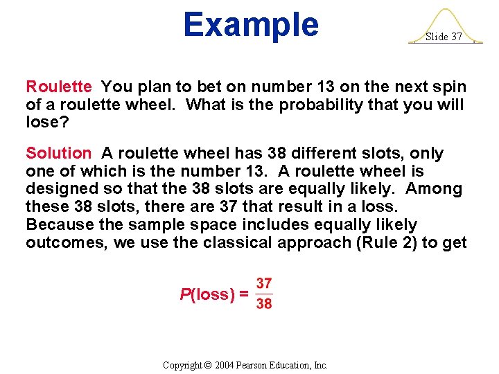
Example Slide 37 Roulette You plan to bet on number 13 on the next spin of a roulette wheel. What is the probability that you will lose? Solution A roulette wheel has 38 different slots, only one of which is the number 13. A roulette wheel is designed so that the 38 slots are equally likely. Among these 38 slots, there are 37 that result in a loss. Because the sample space includes equally likely outcomes, we use the classical approach (Rule 2) to get P(loss) = Copyright © 2004 Pearson Education, Inc.

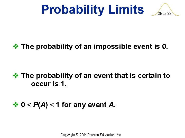
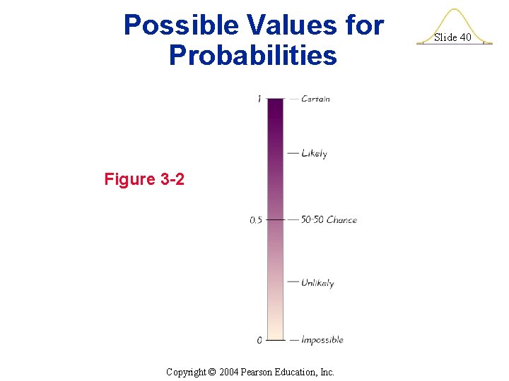
Probability Limits Slide 38 v The probability of an impossible event is 0. v The probability of an event that is certain to occur is 1. v 0 P(A) 1 for any event A. Copyright © 2004 Pearson Education, Inc.

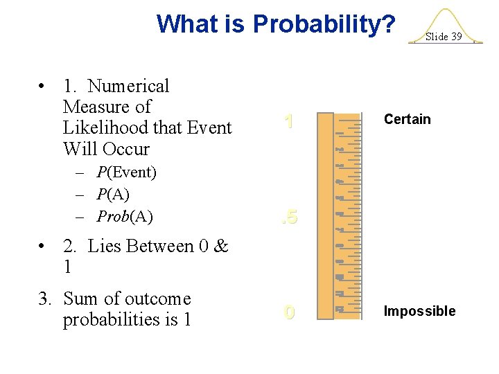
What is Probability? • 1. Numerical Measure of Likelihood that Event Will Occur – P(Event) – P(A) – Prob(A) 1 Slide 39 Certain . 5 • 2. Lies Between 0 & 1 3. Sum of outcome probabilities is 1 0 Impossible

Possible Values for Probabilities Figure 3 -2 Copyright © 2004 Pearson Education, Inc. Slide 40

Definition Slide 41 The complement of event A, denoted by A, consists of all outcomes in which the event A does not occur. Copyright © 2004 Pearson Education, Inc.

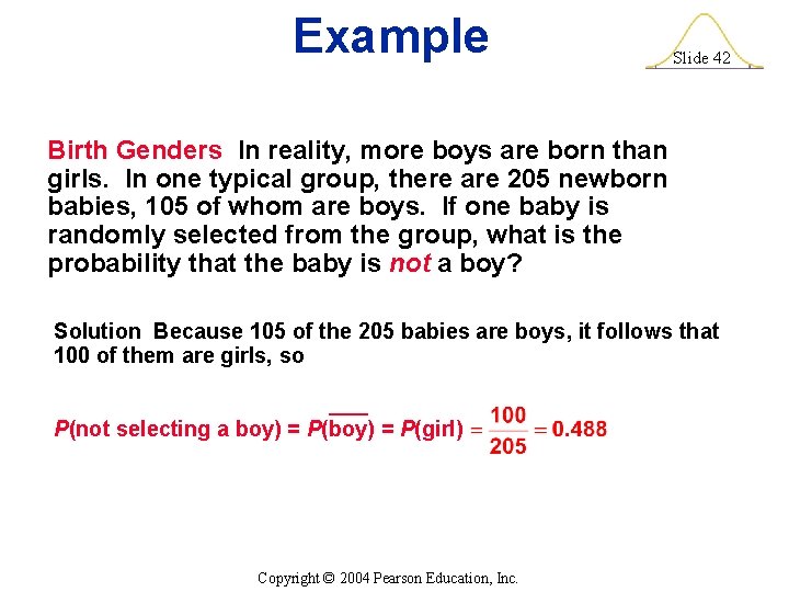
Example Slide 42 Birth Genders In reality, more boys are born than girls. In one typical group, there are 205 newborn babies, 105 of whom are boys. If one baby is randomly selected from the group, what is the probability that the baby is not a boy? Solution Because 105 of the 205 babies are boys, it follows that 100 of them are girls, so P(not selecting a boy) = P(girl) Copyright © 2004 Pearson Education, Inc.

Rounding Off Probabilities Slide 43 When expressing the value of a probability, either give the exact fraction or decimal or round off final decimal results to three significant digits. (Suggestion: When the probability is not a simple fraction such as 2/3 or 5/9, express it as a decimal so that the number can be better understood. ) Copyright © 2004 Pearson Education, Inc.

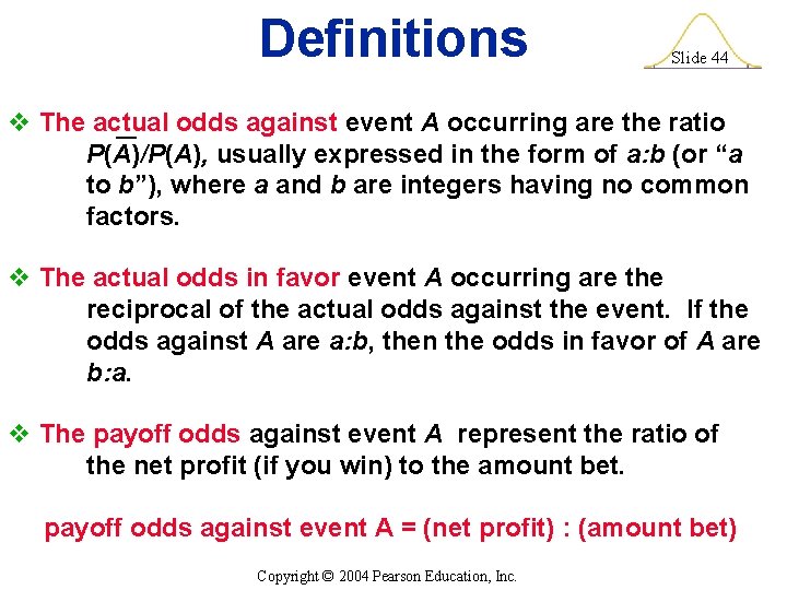
Definitions Slide 44 v The actual odds against event A occurring are the ratio P(A)/P(A), usually expressed in the form of a: b (or “a to b”), where a and b are integers having no common factors. v The actual odds in favor event A occurring are the reciprocal of the actual odds against the event. If the odds against A are a: b, then the odds in favor of A are b: a. v The payoff odds against event A represent the ratio of the net profit (if you win) to the amount bet. payoff odds against event A = (net profit) : (amount bet) Copyright © 2004 Pearson Education, Inc.

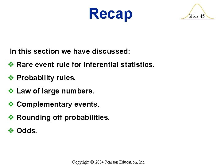
Recap In this section we have discussed: v Rare event rule for inferential statistics. v Probability rules. v Law of large numbers. v Complementary events. v Rounding off probabilities. v Odds. Copyright © 2004 Pearson Education, Inc. Slide 45