Lecture 4 Variability Standard Deviation Variability Reminder How
Lecture 4 Variability: Standard Deviation
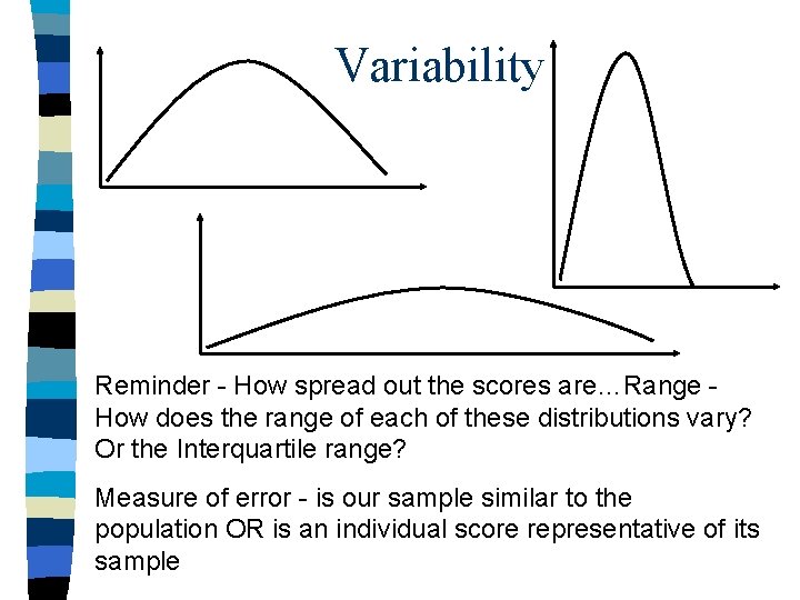
Variability Reminder - How spread out the scores are…Range How does the range of each of these distributions vary? Or the Interquartile range? Measure of error - is our sample similar to the population OR is an individual score representative of its sample
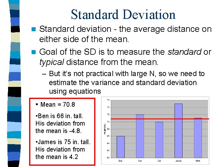
Standard Deviation Standard deviation - the average distance on either side of the mean. n Goal of the SD is to measure the standard or typical distance from the mean. n – But it’s not practical with large N, so we need to estimate the variance and standard deviation using equations • Mean = 70. 8 • Ben is 66 in. tall. His deviation from the mean is -4. 8. • James is 75 in. tall. His deviation from the mean is 4. 2
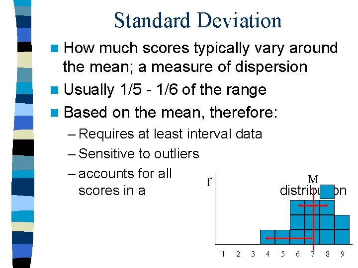
Standard Deviation n How much scores typically vary around the mean; a measure of dispersion n Usually 1/5 - 1/6 of the range n Based on the mean, therefore: – Requires at least interval data – Sensitive to outliers – accounts for all f scores in a 1 2 3 M distribution 4 5 6 7 8 9
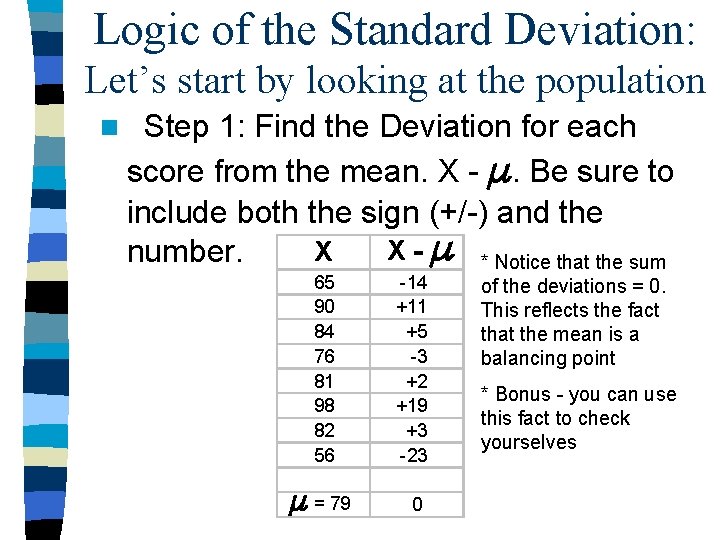
Logic of the Standard Deviation: Let’s start by looking at the population n Step 1: Find the Deviation for each score from the mean. X - . Be sure to include both the sign (+/-) and the X - * Notice that the sum X number. 65 90 84 76 81 98 82 56 -14 +11 +5 -3 +2 +19 +3 -23 = 79 0 of the deviations = 0. This reflects the fact that the mean is a balancing point * Bonus - you can use this fact to check yourselves
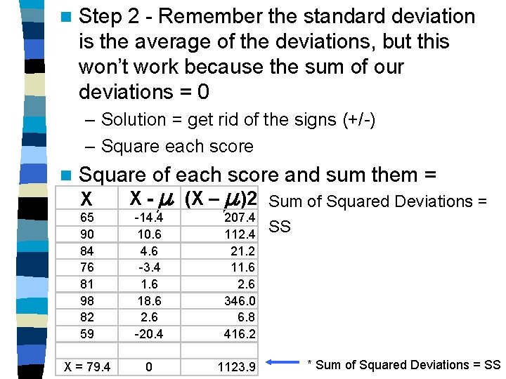
n Step 2 - Remember the standard deviation is the average of the deviations, but this won’t work because the sum of our deviations = 0 – Solution = get rid of the signs (+/-) – Square each score n Square of each score and sum them = X 65 90 84 76 81 98 82 59 X = 79. 4 X - (X – )2 Sum of Squared Deviations = -14. 4 10. 6 4. 6 -3. 4 1. 6 18. 6 2. 6 -20. 4 207. 4 112. 4 21. 2 11. 6 2. 6 346. 0 6. 8 416. 2 0 1123. 9 SS * Sum of Squared Deviations = SS
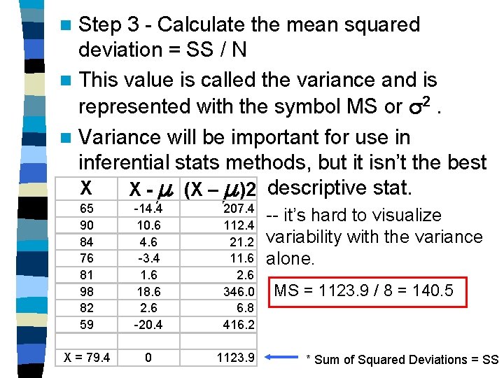
Step 3 - Calculate the mean squared deviation = SS / N n This value is called the variance and is represented with the symbol MS or 2. n Variance will be important for use in inferential stats methods, but it isn’t the best X X - (X – )2 descriptive stat. n 65 90 84 76 81 98 82 59 -14. 4 10. 6 4. 6 -3. 4 1. 6 18. 6 2. 6 -20. 4 207. 4 112. 4 21. 2 11. 6 2. 6 346. 0 6. 8 416. 2 X = 79. 4 0 1123. 9 -- it’s hard to visualize variability with the variance alone. MS = 1123. 9 / 8 = 140. 5 * Sum of Squared Deviations = SS
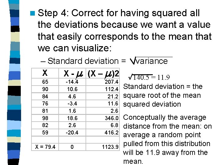
n Step 4: Correct for having squared all the deviations because we want a value that easily corresponds to the mean that we can visualize: – Standard deviation = X 65 90 84 76 81 98 82 59 X = 79. 4 X - (X – )2 -14. 4 10. 6 4. 6 -3. 4 1. 6 18. 6 2. 6 -20. 4 207. 4 112. 4 21. 2 11. 6 2. 6 346. 0 6. 8 416. 2 0 1123. 9 variance 140. 5 = 11. 9 Standard deviation = the square root of the mean squared deviation Conceptually the average distance from the mean: on average a random point pulled from this distribution will be 11. 9 away from the mean.
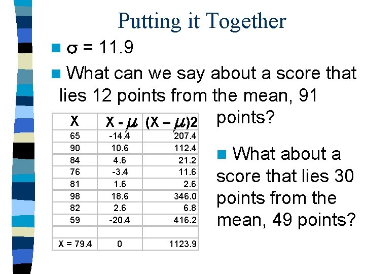
Putting it Together = 11. 9 n What can we say about a score that lies 12 points from the mean, 91 X X - (X – )2 points? n 65 90 84 76 81 98 82 59 -14. 4 10. 6 4. 6 -3. 4 1. 6 18. 6 2. 6 -20. 4 207. 4 112. 4 21. 2 11. 6 2. 6 346. 0 6. 8 416. 2 X = 79. 4 0 1123. 9 What about a score that lies 30 points from the mean, 49 points? n
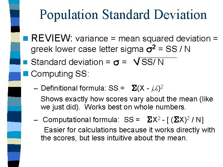
Population Standard Deviation n REVIEW: variance = mean squared deviation = greek lower case letter sigma 2 = SS / N Standard deviation = = n Computing SS: n SS/ N – Definitional formula: SS = (X - )2 Shows exactly how scores vary about the mean (like we just did). Works best on whole numbers. – Computational formula: SS = X 2 - [ ( X)2 / N] Easier for calculations because it works directly with the scores, but less intuitive about the mean.
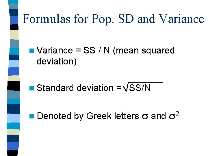
Formulas for Pop. SD and Variance n Variance = SS / N (mean squared deviation) n Standard n Denoted deviation = SS/N by Greek letters and 2
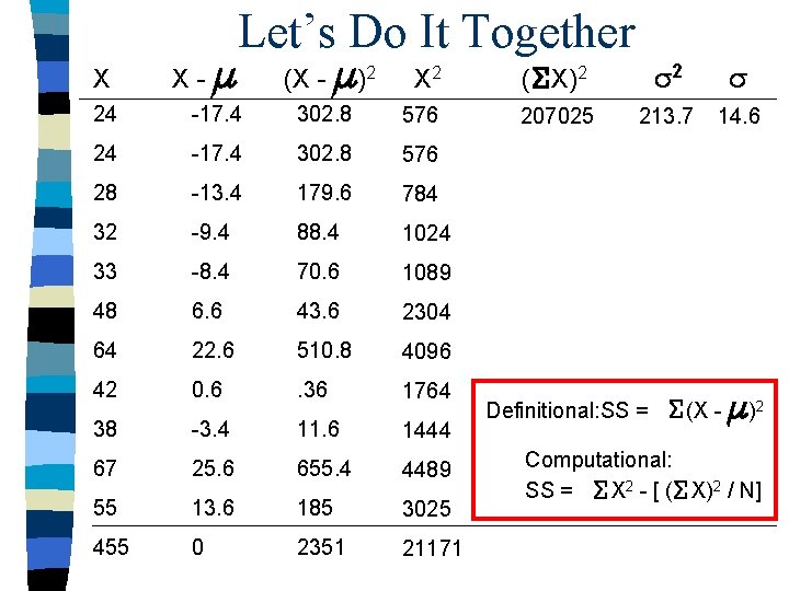
X X- Let’s Do It Together (X - )2 X 2 ( X)2 2 207025 213. 7 14. 6 24 -17. 4 302. 8 576 28 -13. 4 179. 6 784 32 -9. 4 88. 4 1024 33 -8. 4 70. 6 1089 48 6. 6 43. 6 2304 64 22. 6 510. 8 4096 42 0. 6 . 36 1764 38 -3. 4 11. 6 1444 67 25. 6 655. 4 4489 55 13. 6 185 3025 455 0 2351 21171 Definitional: SS = (X - )2 Computational: SS = X 2 - [ ( X)2 / N]
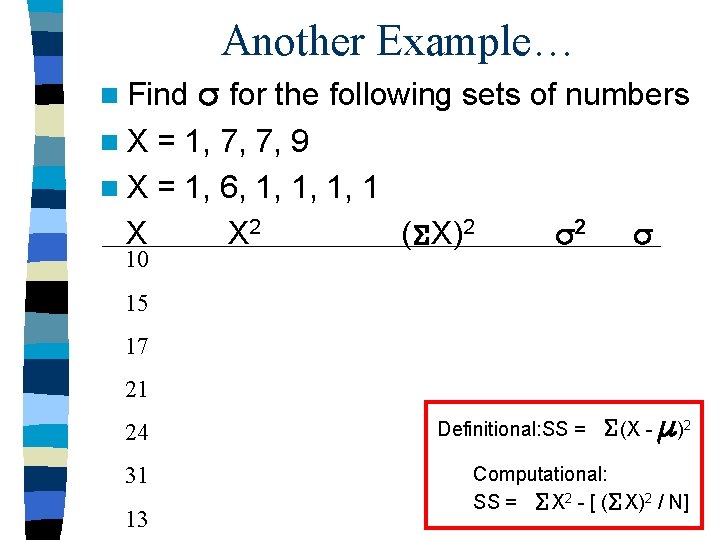
Another Example… n Find for the following sets of numbers n. X = 1, 7, 7, 9 n X = 1, 6, 1, 1 X X 2 ( X)2 10 2 15 17 21 24 31 13 Definitional: SS = (X - )2 Computational: SS = X 2 - [ ( X)2 / N]
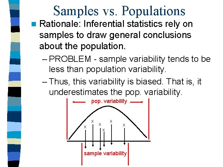
Samples vs. Populations n Rationale: Inferential statistics rely on samples to draw general conclusions about the population. – PROBLEM - sample variability tends to be less than population variability. – Thus, this variability is biased. That is, it underestimates the pop. variability x x x sample variability
Terms n Biased - a sample statistic is said to be biased if on the average the sample statistic consistently underestimates or overestimates the population parameter. n Unbiased - a sample statistic is said to be unbiased if on average the sample statistics is equal to the population parameter
An Analogy for a Biased Stat n Imagine you were interested in studying learning in elementary school children. – What if you chose as your sample child geniuses from computer and science camp? – Could you generalize from your sample to the population of elementary school children? n. A sample statistic for SD will be biased even with a representative sample - We have to perform a correction
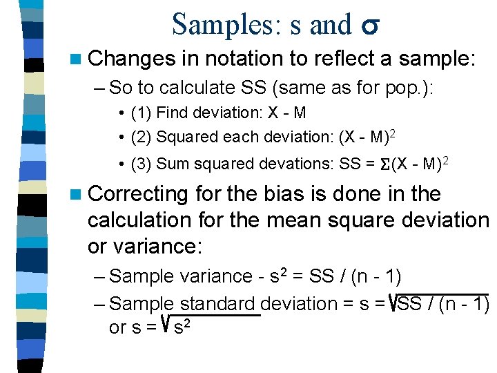
Samples: s and n Changes in notation to reflect a sample: – So to calculate SS (same as for pop. ): • (1) Find deviation: X - M • (2) Squared each deviation: (X - M)2 • (3) Sum squared devations: SS = (X - M)2 n Correcting for the bias is done in the calculation for the mean square deviation or variance: – Sample variance - s 2 = SS / (n - 1) – Sample standard deviation = s = SS / (n - 1) or s = s 2
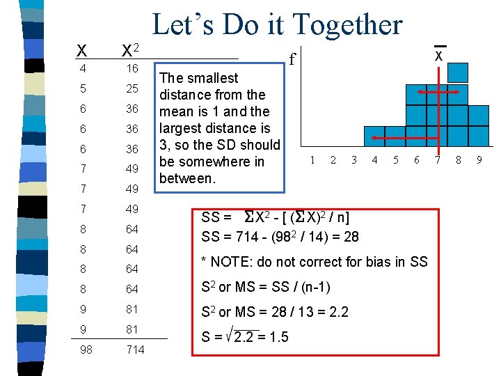
Let’s Do it Together X X 2 4 16 5 25 6 36 7 49 8 64 S 2 or MS = SS / (n-1) 9 81 S 2 or MS = 28 / 13 = 2. 2 9 81 98 714 X f The smallest distance from the mean is 1 and the largest distance is 3, so the SD should be somewhere in between. 1 2 3 4 5 6 SS = X 2 - [ ( X)2 / n] SS = 714 - (982 / 14) = 28 * NOTE: do not correct for bias in SS S = 2. 2 = 1. 5 7 8 9
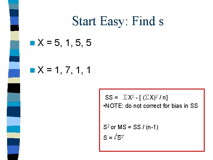
Start Easy: Find s n. X = 5, 1, 5, 5 n. X = 1, 7, 1, 1 SS = X 2 - [ ( X)2 / n] • NOTE: do not correct for bias in SS S 2 or MS = SS / (n-1) S = S 2
![A little more complex SS = X 2 - [ ( X)2 / n] A little more complex SS = X 2 - [ ( X)2 / n]](http://slidetodoc.com/presentation_image_h/3104351e0b88d87476a91a3ca42a9d44/image-20.jpg)
A little more complex SS = X 2 - [ ( X)2 / n] MS or S 2 = SS / n-1 s = SS / (n - 1) SS = 1698474. 01 - (26005920. 2 / 16) MS = 73104 / 15 s = 69. 8 5099. 6 1698474. 01
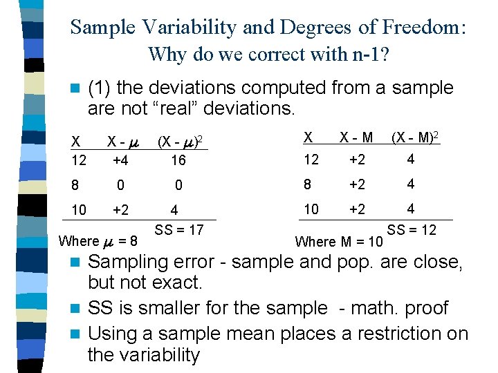
Sample Variability and Degrees of Freedom: Why do we correct with n-1? n (1) the deviations computed from a sample are not “real” deviations. X X-M (X - M)2 12 +2 4 X 12 X- +4 (X - 16 8 0 0 8 +2 4 10 +2 4 SS = 17 10 +2 4 Where = 8 )2 Where M = 10 SS = 12 Sampling error - sample and pop. are close, but not exact. n SS is smaller for the sample - math. proof n Using a sample mean places a restriction on the variability n
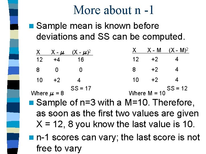
More about n -1 n Sample mean is known before deviations and SS can be computed. X 12 X- +4 (X - )2 16 X X-M (X - M)2 12 +2 4 8 0 0 8 +2 4 10 +2 4 SS = 17 10 +2 4 Where = 8 n Sample Where M = 10 SS = 12 of n=3 with a M=10. Therefore, as soon as the first two values are given X = 12, 8 you know the last value is 10. n n-1 scores can vary; the last score is not free to vary
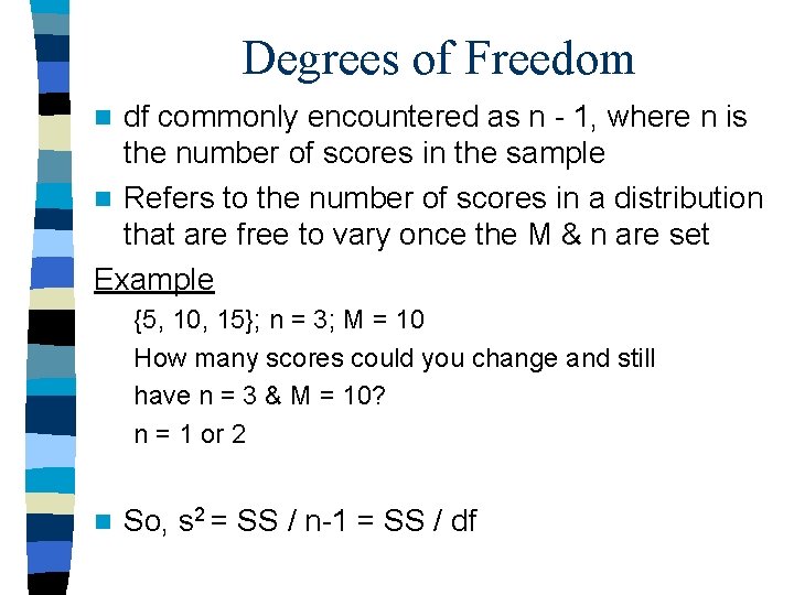
Degrees of Freedom df commonly encountered as n - 1, where n is the number of scores in the sample n Refers to the number of scores in a distribution that are free to vary once the M & n are set Example n {5, 10, 15}; n = 3; M = 10 How many scores could you change and still have n = 3 & M = 10? n = 1 or 2 n So, s 2 = SS / n-1 = SS / df
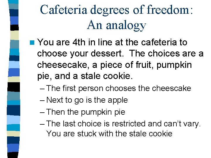
Cafeteria degrees of freedom: An analogy n You are 4 th in line at the cafeteria to choose your dessert. The choices are a cheesecake, a piece of fruit, pumpkin pie, and a stale cookie. – The first person chooses the cheescake – Next to go is the apple – Then the pumpkin pie – The last choice is restricted and can’t vary. You are stuck with the stale cookie
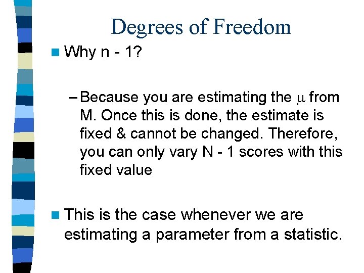
Degrees of Freedom n Why n - 1? – Because you are estimating the from M. Once this is done, the estimate is fixed & cannot be changed. Therefore, you can only vary N - 1 scores with this fixed value n This is the case whenever we are estimating a parameter from a statistic.
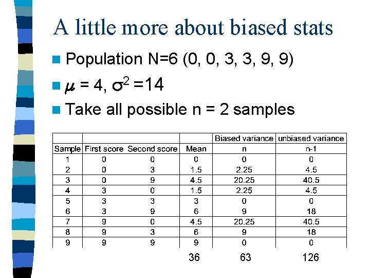
A little more about biased stats n Population N=6 (0, 0, 3, 3, 9, 9) = 4, 2 =14 n Take all possible n = 2 samples n 36 63 126
Properties of the Standard Deviation n Distribution: – Homogeneous sample: data values are very similar = small s 2 and s. – Heterogeneous sample: data values are dissimilar = big s 2 and s. n Helps make predictions about the amount of error in your sample. How close is your sample to the population
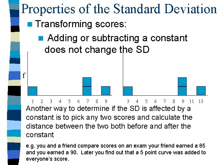
Properties of the Standard Deviation n Transforming scores: n Adding or subtracting a constant does not change the SD f 1 2 3 4 5 6 7 8 9 11 13 Another way to determine if the SD is affected by a constant is to pick any two scores and calculate the distance between the two both before and after the constant e. g. you and a friend compare scores on an exam your friend earned a 85 and you earned a 90. Later you find out that a 5 point curve was added to everyone’s score.
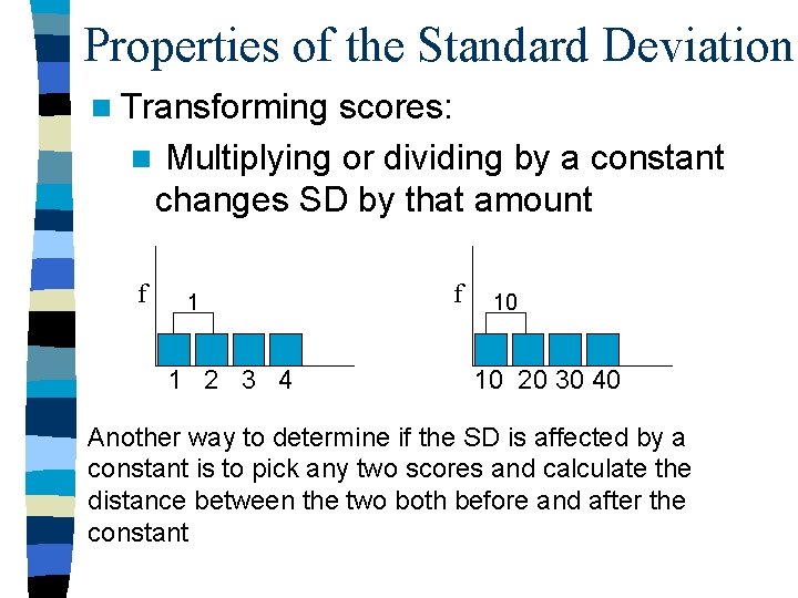
Properties of the Standard Deviation n Transforming scores: n Multiplying or dividing by a constant changes SD by that amount f 1 1 2 3 4 f 10 10 20 30 40 Another way to determine if the SD is affected by a constant is to pick any two scores and calculate the distance between the two both before and after the constant
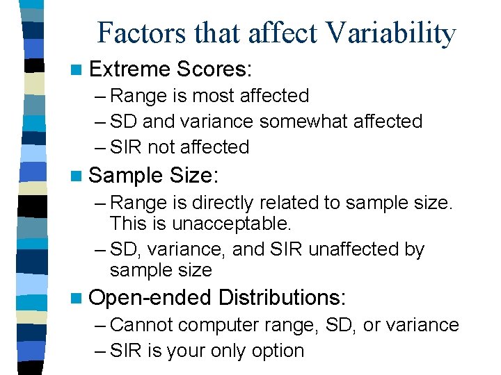
Factors that affect Variability n Extreme Scores: – Range is most affected – SD and variance somewhat affected – SIR not affected n Sample Size: – Range is directly related to sample size. This is unacceptable. – SD, variance, and SIR unaffected by sample size n Open-ended Distributions: – Cannot computer range, SD, or variance – SIR is your only option
Relationship with other Statistics n SD is derived using information about the mean (distances) - the two go handin-hand n Interquartile range (& SIR) are based on percentiles, so is the median (mdn is 50 th percentile) n Range has no direct relationship with any other statistical measures
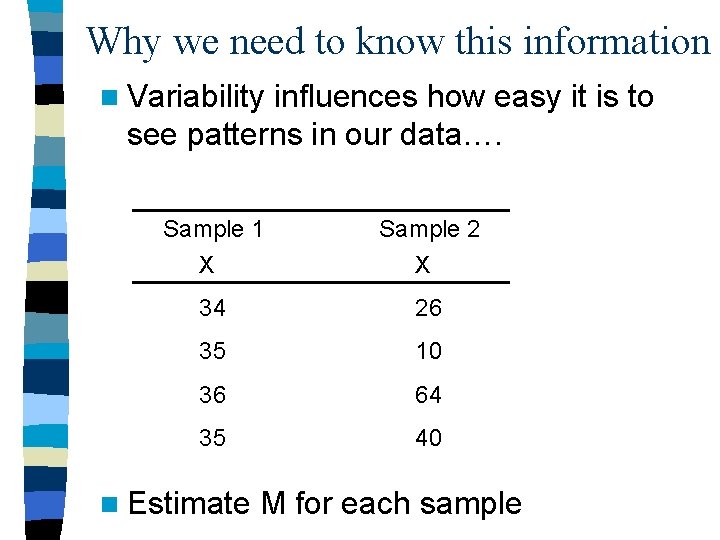
Why we need to know this information n Variability influences how easy it is to see patterns in our data…. Sample 1 X Sample 2 X 34 26 35 10 36 64 35 40 n Estimate M for each sample
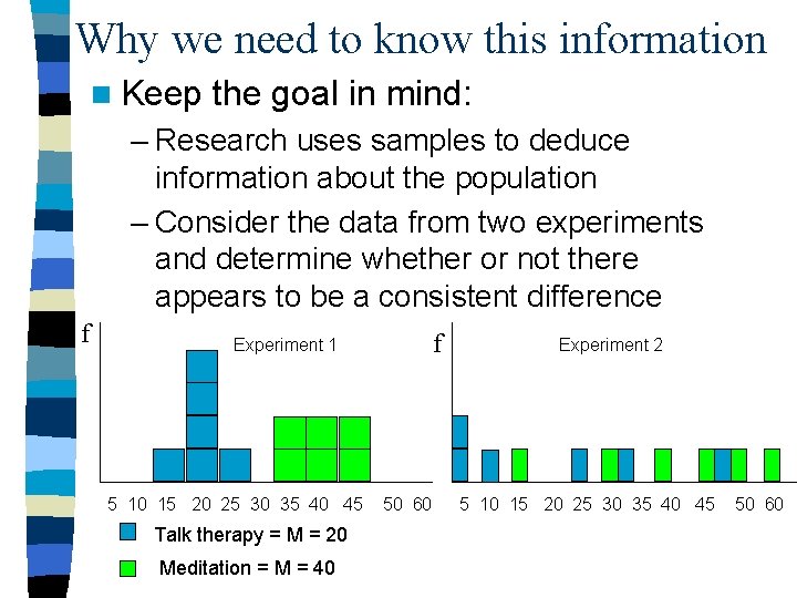
Why we need to know this information n Keep the goal in mind: – Research uses samples to deduce information about the population – Consider the data from two experiments and determine whether or not there appears to be a consistent difference f f Experiment 1 5 10 15 20 25 30 35 40 45 Talk therapy = M = 20 Meditation = M = 40 50 60 Experiment 2 5 10 15 20 25 30 35 40 45 50 60
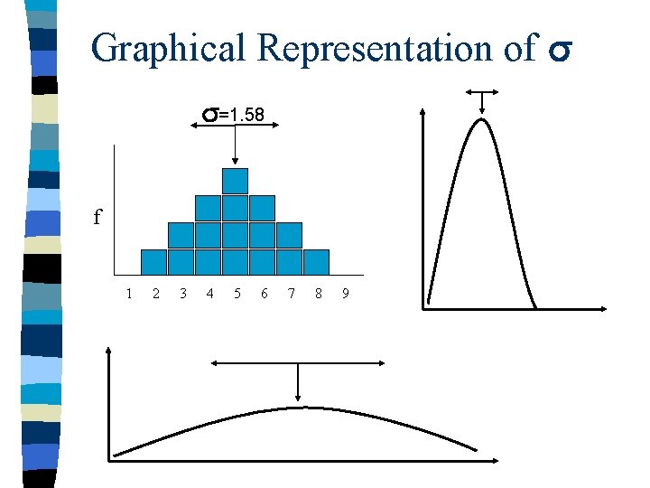
Graphical Representation of =1. 58 f 1 2 3 4 5 6 7 8 9
Graphic Representation - Box Plots Also called box-and-whisker plots n Useful for n – comparing distributions – displaying variability n Box defines the interquartile range – Top line defines the third quartile – Bottom line defines the first quartile n Whiskers extend out to the highest and lowest scores n Median is often displayed by a line
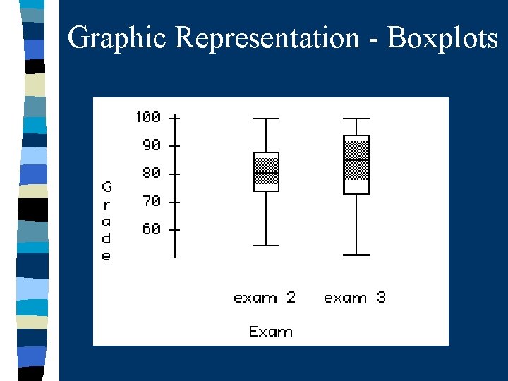
Graphic Representation - Boxplots
Pearson’s Coefficient of Skew n Pearson’s coefficient of skew tells us if a distribution is positive or negatively skewed and how much (+/- 0. 5 is approximately symmetric/normal) n s 3 = [3(M - mdn)] / s n M = 20, s = 5, md = 24 n s 3 = [3(20 - 24)] / 5 s 3 = -2. 4 n Negatively skewed
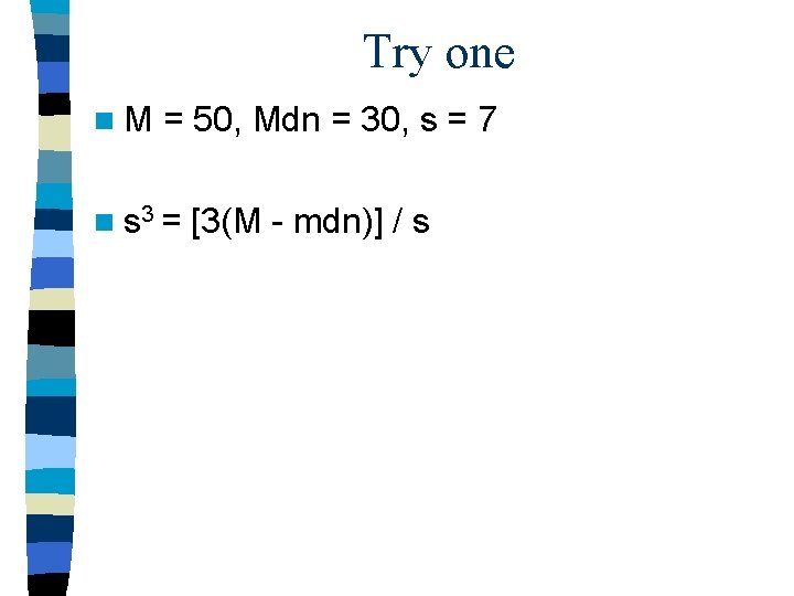
Try one n. M = 50, Mdn = 30, s = 7 n s 3 = [3(M - mdn)] / s
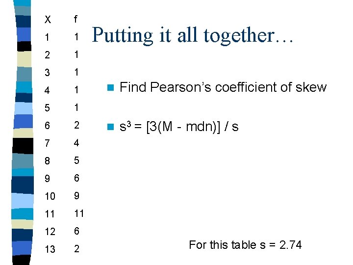
X f 1 1 2 1 3 1 4 1 5 1 6 2 7 4 8 5 9 6 10 9 11 11 12 6 13 2 Putting it all together… n Find Pearson’s coefficient of skew n s 3 = [3(M - mdn)] / s For this table s = 2. 74

Homework: Chapter 4 n 1, 3, 4, 6, 8, 11, 12, 14, 19, 20, 23, 24, 25 n Read IN THE LITERATURE pg 122 -123. n Skim Chapter 6 pages 161 - 166; section on Probability. n ** BRING YOUR TEXT BOOKS TO CLASS TOMORROW**
- Slides: 40