Lecture 4 Structure plan n Program design process

Lecture 4 Structure plan n. Program design process n. Basic elements of code: –Input (assignment of variables) –Sequence of expressions –Output (graphical or tabular) n. Structured approach to design © 2007 Daniel Valentine. All rights reserved. Published by Elsevier.

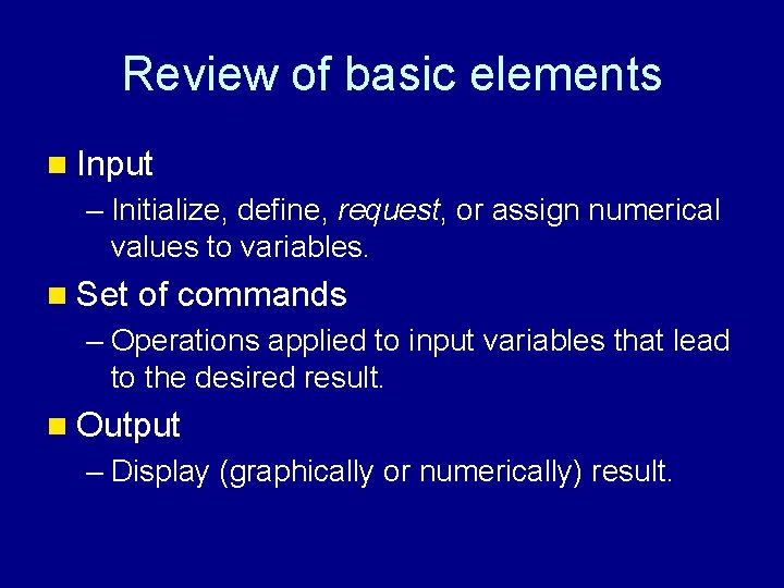
Review of basic elements n Input – Initialize, define, request, or assign numerical values to variables. n Set of commands – Operations applied to input variables that lead to the desired result. n Output – Display (graphically or numerically) result.

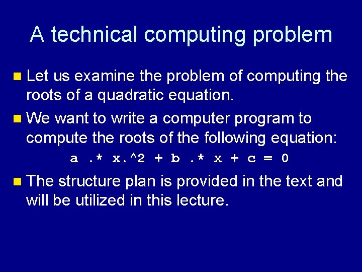
A technical computing problem n Let us examine the problem of computing the roots of a quadratic equation. n We want to write a computer program to compute the roots of the following equation: a. * x. ^2 + b. * x + c = 0 n The structure plan is provided in the text and will be utilized in this lecture.

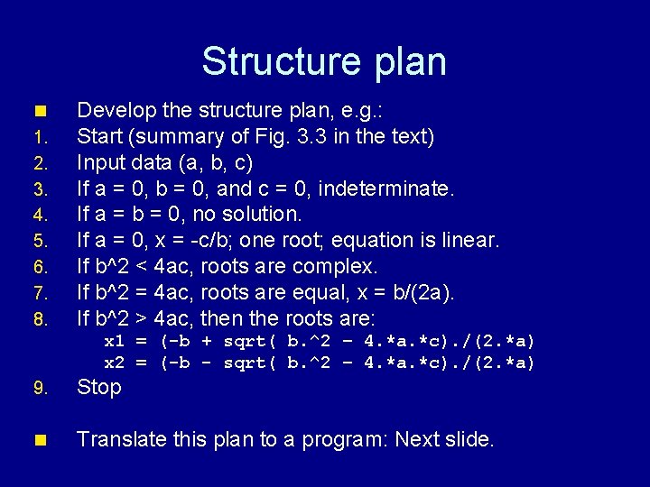
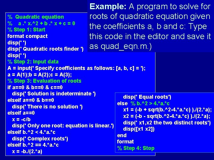
Structure plan n 1. 2. 3. 4. 5. 6. 7. 8. Develop the structure plan, e. g. : Start (summary of Fig. 3. 3 in the text) Input data (a, b, c) If a = 0, b = 0, and c = 0, indeterminate. If a = b = 0, no solution. If a = 0, x = -c/b; one root; equation is linear. If b^2 < 4 ac, roots are complex. If b^2 = 4 ac, roots are equal, x = b/(2 a). If b^2 > 4 ac, then the roots are: x 1 x 2 = = (-b + - sqrt( b. ^2 – – 4. *a. *c). /(2. *a) 9. Stop n Translate this plan to a program: Next slide.

Example: A program to solve for roots of quadratic equation given the coefficients a, b and c: Type this code in the editor and save it as quad_eqn. m. ) % Quadratic equation % a. * x. ^2 + b. * x + c = 0 % Step 1: Start format compact disp(' ') disp(' Quadratic roots finder ') disp(' ') % Step 2: Input data A = input(' Specify coefficients as follows: [a, b, c] = '); a = A(1); b = A(2); c = A(3); % Step 3: Evaluation of roots if a==0 & b==0 & c==0 disp(' Solution is indeterminate ') disp(' Equal roots') elseif a==0 & b==0 else % b. ^2 > 4. *a. *c disp(' There is no solution ') x 1 = (-b + sqrt(b. ^2 -4. *a. *c) ). /(2. *a); elseif a==0 x 2 = (-b - sqrt(b. ^2 -4. *a. *c) ). /(2. *a); x = -c/b disp(' x 1, x 2 the two distinct roots') disp(' Only one root: equation is linear. ') disp([x 1 x 2]) elseif b. ^2 < 4. *a. *c end disp(' Complex roots') format elseif b. ^2 == 4. *a. *c % Step 4: Stop x = -b. /(2. *a)

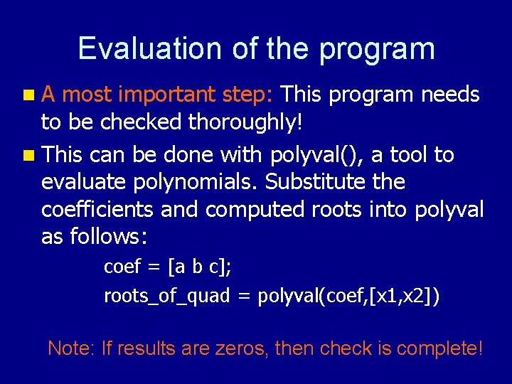
Evaluation of the program n. A most important step: This program needs to be checked thoroughly! n This can be done with polyval(), a tool to evaluate polynomials. Substitute the coefficients and computed roots into polyval as follows: coef = [a b c]; roots_of_quad = polyval(coef, [x 1, x 2]) Note: If results are zeros, then check is complete!

Exercise n Evaluate the quad_eqn. m program as described in the previous slide: See next slide. n Executing the program numerous times evaluating the results and comparing with known answers is important. You must be convinced, that every time you use the code to compute roots of a quadratic equation, it does it correctly!

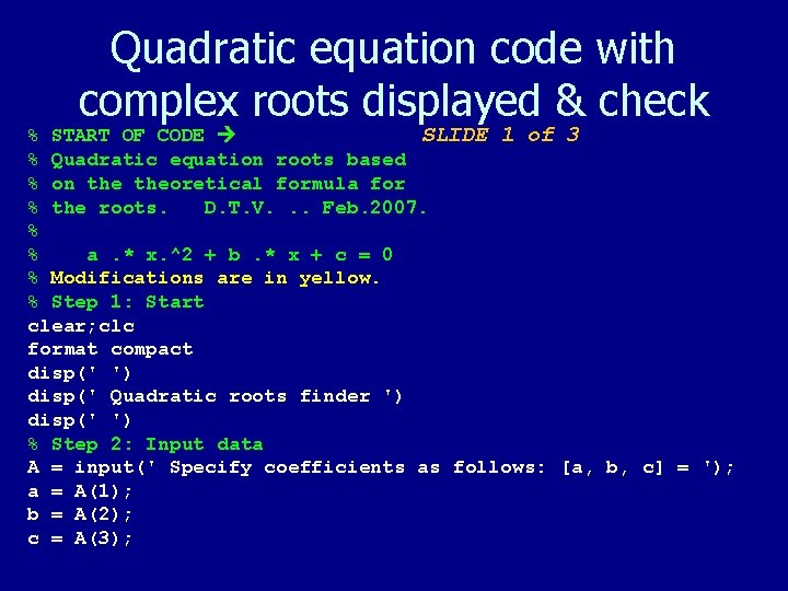
Quadratic equation code with complex roots displayed & check % START OF CODE SLIDE 1 of 3 % Quadratic equation roots based % on theoretical formula for % the roots. D. T. V. . . Feb. 2007. % % a. * x. ^2 + b. * x + c = 0 % Modifications are in yellow. % Step 1: Start clear; clc format compact disp(' ') disp(' Quadratic roots finder ') disp(' ') % Step 2: Input data A = input(' Specify coefficients as follows: [a, b, c] = '); a = A(1); b = A(2); c = A(3);

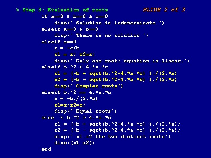
% Step 3: Evaluation of roots SLIDE 2 of 3 if a==0 & b==0 & c==0 disp(' Solution is indeterminate ') elseif a==0 & b==0 disp(' There is no solution ') elseif a==0 x = -c/b x 1 = x; x 2=x; disp(' Only one root: equation is linear. ') elseif b. ^2 < 4. *a. *c x 1 = (-b + sqrt(b. ^2 -4. *a. *c) ). /(2. *a) x 2 = (-b - sqrt(b. ^2 -4. *a. *c) ). /(2. *a) disp(' Complex roots') elseif b. ^2 == 4. *a. *c x = -b. /(2. *a) x 1=x; x 2=x; disp(' Equal roots') else % b. ^2 > 4. *a. *c x 1 = (-b + sqrt(b. ^2 -4. *a. *c) ). /(2. *a); x 2 = (-b - sqrt(b. ^2 -4. *a. *c) ). /(2. *a); disp(' x 1, x 2 the two distinct roots') disp([x 1 x 2]) end

This is the check at the end: format disp('check') coef = [a b c]; roots_of_quad = polyval(coef, [x 1, x 2]) % Step 4: Stop SLIDE 3 of 3 Note: Evaluation and validation of a computer program is the most time consuming and necessary effort to ensure that the tool produces reliable and correct results.

Summary n The structure plan approach to design computer codes for technical computing was introduced by an example. n Input assignment was illustrated with and without the ‘input’ utility. n Graphical & tabular forms of output were shown. n Illustrated array dot-operation, repetition (for) and decision (if) programming tools.