Lecture 4 Simulation of Queueing System Single channel

Lecture 4 Simulation of Queueing System Single channel Queue

Simulation of Queueing Systems Example: Single-Channel Queue § Assumptions • Only one checkout counter. • Customers arrive at this checkout counter at random from 1 to 8 minutes apart. Each possible value of interarrival time has the same probability of occurrence, as shown in Table 2. 6. • The service times vary from 1 to 6 minutes with the probabilities shown in Table 2. 7. • The problem is to analyze the system by simulating the arrival and service of 20 customers.

Simulation of Queueing Systems

Simulation of Queueing Systems Example (Cont. ) n n A simulation of a grocery store that starts with an empty system is not realistic unless the intention is to model the system from startup or to model until steady-state operation is reached. A set of uniformly distributed random numbers is needed to generate the arrivals at the checkout counter. Random numbers have the following properties: w The set of random numbers is uniformly distributed between 0 and 1. w Successive random numbers are independent. n n Random digits are converted to random numbers by placing a decimal point appropriately. The rightmost two columns of Tables 2. 6 and 2. 7 are used to generate random arrivals and random service times.

Simulation of Queueing Systems Example (Cont. ) Table 2. 8 n The first random digits are 913. To obtain the corresponding time between arrivals, enter the fourth column of Table 2. 6 and read 8 minutes from the first column of the table.

Simulation of Queueing Systems Example (Cont. ) Table 2. 9 n The first customer's service time is 4 minutes because the random digits 84 fall in the bracket 61 -85

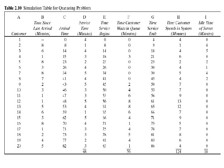
Simulation of Queueing Systems Example (Cont. ) n n The essence of a manual simulation is the simulation table. The simulation table for the single-channel queue, shown in Table 2. 10, is an extension of the type of table already seen in Table 2. 4. Statistical measures of performance can be obtained form the simulation table such as Table 2. 10. Statistical measures of performance in this example. w Each customer's time in the system w The server's idle time n In order to compute summary statistics, totals are formed as shown for service times, time customers spend in the system, idle time of the server, and time the customers wait in the queue.

Simulation of Queueing Systems Example (Cont. ) n The average waiting time for a customer : 2. 8 minutes n The probability that a customer has to wait in the queue : 0. 65 n The fraction of idle time of the server : 0. 21 n The probability of the server being busy: 0. 79 (=1 -0. 21)

Simulation of Queueing Systems Example (Cont. ) n The average service time : 3. 4 minutes This result can be compared with the expected service time by finding the mean of the service-time distribution using the equation in table 2. 7. The expected service time is slightly lower than the average service time in the simulation. The longer the simulation, the closer the average will be to

Simulation of Queueing Systems Example (Cont. ) n n The average time between arrivals : 4. 3 minutes This result can be compared to the expected time between arrivals by finding the mean of the discrete uniform distribution whose endpoints are a=1 and b=8. The longer the simulation, the closer the average will be to n The average waiting time of those who wait : 4. 3 minutes

Simulation of Queueing Systems Example (Cont. ) n The average time a customer spends in the system : 6. 2 minutes average time customer spends in the system = average time customer spends + customer spends waiting in the queue in service average time customer spends in the system = 2. 8 + 3. 4 = 6. 2 (min)

Simulation of Queueing Systems Example: The Able Baker Carhop Problem § A drive-in restaurant where carhops take orders and bring food to the car. § Assumptions • Cars arrive in the manner shown in Table 2. 11. • Two carhops Able and Baker - Able is better able to do the job and works a bit faster than Baker. • The distribution of their service times is shown in Tables 2. 12 and 2. 13.

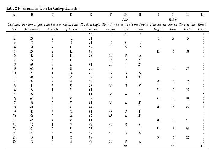
Simulation of Queueing Systems Example: (Cont. ) n n A simplifying rule is that Able gets the customer if both carhops are idle. If both are busy, the customer begins service with the first server to become free. To estimate the system measures of performance, a simulation of 1 hour of operation is made. The problem is to find how well the current arrangement is working.

Simulation of Queueing Systems Example 2. 2 (cont. ) n The row for the first customer is filled in manually, with the randomnumber function RAND() in case of Excel or another random function replacing the random digits. n After the first customer, the cells for the other customers must be based on logic and formulas. For example, the “Clock Time of Arrival” (column D) in the row for the second customer is computed as follows: D 2 = D 1 + C 2 n The logic to computer who gets a given customer can use the Excel macro function IF(), which returns one of two values depending on whether a condition is true or false. IF( condition, value if true, value if false)

clock = 0 Is it time of arrival? Yes Is Able idle? No Is Baker idle? No Nothing No Yes Is there the service completed? Yes Store clock time (column H or K) service (column E) Generate random digit for Convert random digit to random number for service time (column G) Able service begin (column F) Generate random digit for service (column E) Convert random digit to random (column J) number for service time Baker service begin (column I) No Increment clock

Simulation of Queueing Systems The analysis of Table 2. 14 results in the following: n Over the 62 -minute period Able was busy 90% of the time. n Baker was busy only 69% of the time. The seniority rule keeps Baker less busy (and gives Able more tips). n Nine of the 26 arrivals (about 35%) had to wait. The average waiting time for all customers was only about 0. 42 minute (25 seconds), which is very small. n Those nine who did have to wait only waited an average of 1. 22 minutes, which is quite low. n In summary, this system seems well balanced. One server cannot handle all the diners, and three servers would probably be too many. Adding an additional server would surely reduce the waiting time to nearly zero. However, the cost of waiting would have to be quite high to justify an additional server.