Lecture 4 Practical Examples Remember this mest m

Lecture 4: Practical Examples

Remember this? mest = m. A + M [ dobs – Gm. A] where M = [GTCd-1 G + Cm-1]-1 GT Cd-1

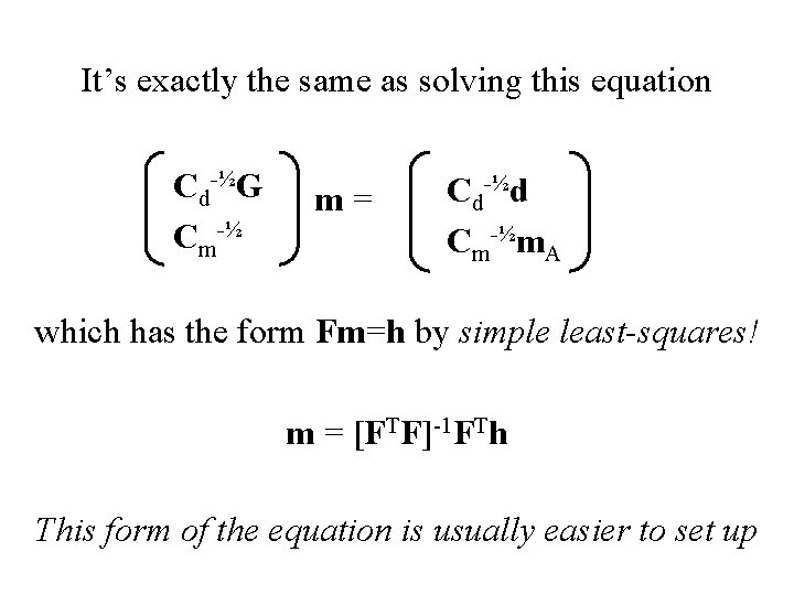
It’s exactly the same as solving this equation Cd-½G Cm-½ m= Cd-½d Cm-½m. A which has the form Fm=h by simple least-squares! m = [FTF]-1 FTh This form of the equation is usually easier to set up

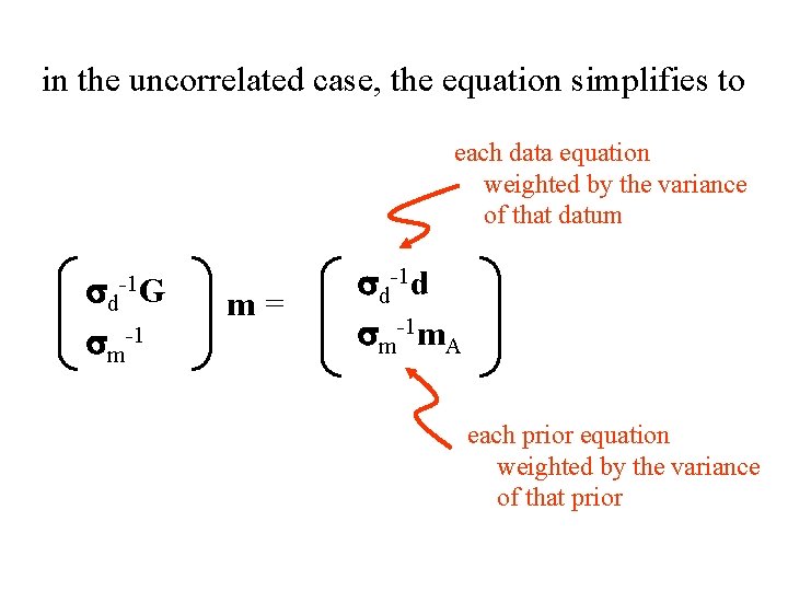
in the uncorrelated case, the equation simplifies to each data equation weighted by the variance of that datum sd-1 G sm-1 m= sd-1 d sm-1 m. A each prior equation weighted by the variance of that prior

Example 1 1 D Interpolation

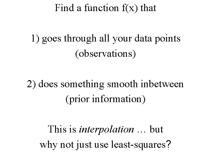
Find a function f(x) that 1) goes through all your data points (observations) 2) does something smooth inbetween (prior information) This is interpolation … but why not just use least-squares?

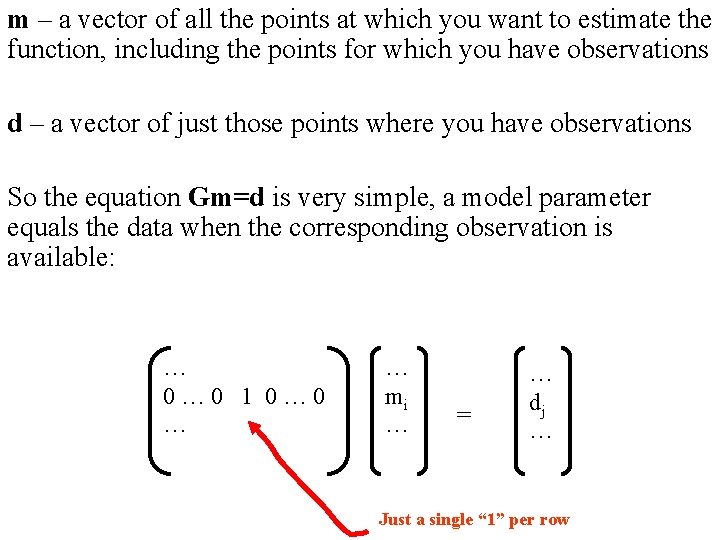
m – a vector of all the points at which you want to estimate the function, including the points for which you have observations d – a vector of just those points where you have observations So the equation Gm=d is very simple, a model parameter equals the data when the corresponding observation is available: … 0… 0 1 0… 0 … … mi … = … dj … Just a single “ 1” per row

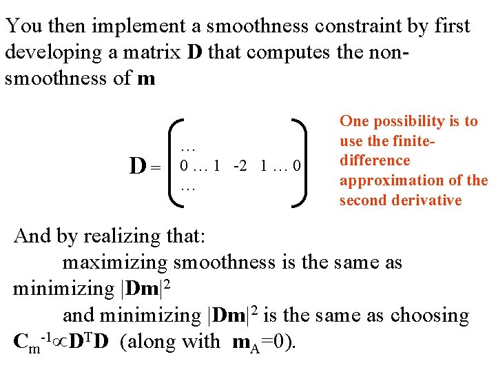
You then implement a smoothness constraint by first developing a matrix D that computes the nonsmoothness of m D= … 0 … 1 -2 1 … 0 … One possibility is to use the finitedifference approximation of the second derivative And by realizing that: maximizing smoothness is the same as minimizing |Dm|2 and minimizing |Dm|2 is the same as choosing Cm-1 DTD (along with m. A=0).

First derivative [dm/dx]i (1/Dx) mi – mi-1 Second derivative [d 2 m/dx 2]i [dm/dx]i+1 - [dm/dx]i = mi+1 – mi + mi-1 = mi+1 – 2 mi + mi-1

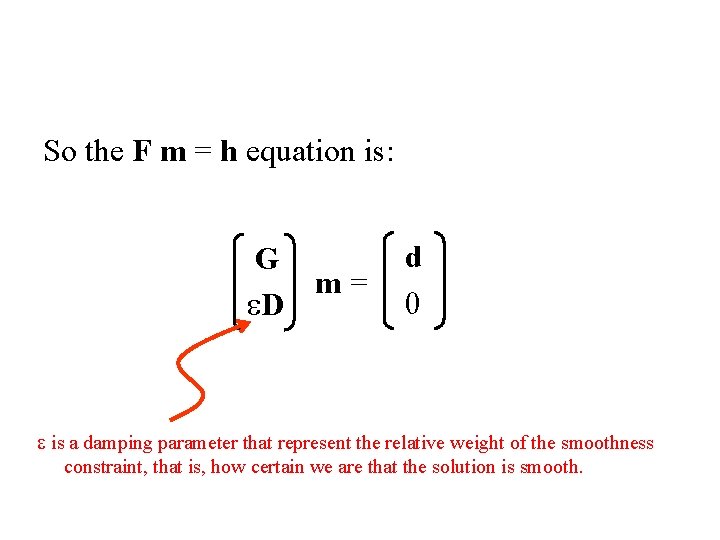
So the F m = h equation is: G m= e. D d 0 e is a damping parameter that represent the relative weight of the smoothness constraint, that is, how certain we are that the solution is smooth.

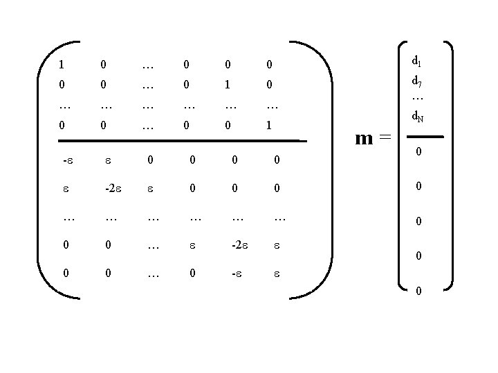
1 0 … 0 0 0 d 1 0 0 … 0 1 0 … … … d 7 … 0 0 1 d. N m= 0 -e e 0 0 e -2 e e 0 0 … … … 0 0 0 … e -2 e e 0 0 … 0 -e e 0 0

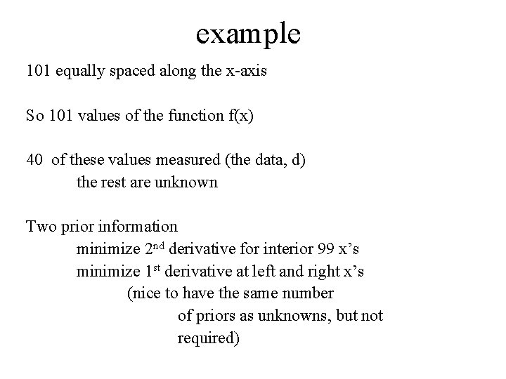
example 101 equally spaced along the x-axis So 101 values of the function f(x) 40 of these values measured (the data, d) the rest are unknown Two prior information minimize 2 nd derivative for interior 99 x’s minimize 1 st derivative at left and right x’s (nice to have the same number of priors as unknowns, but not required)

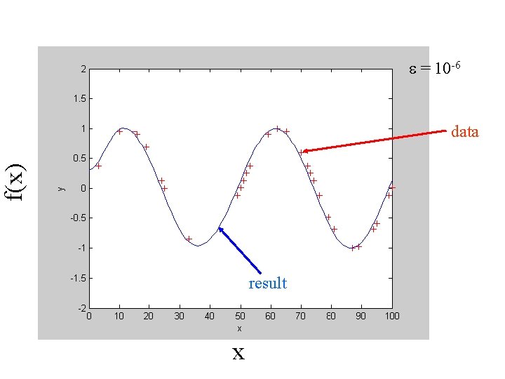
e = 10 -6 f(x) data result x

e can be chosen by trial and error but usually the result fairly insensitive to e, as long as its small

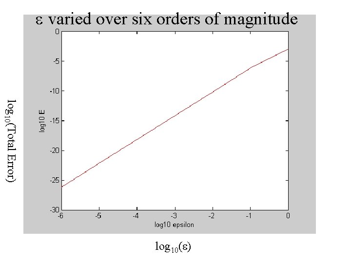
e varied over six orders of magnitude log 10(Total Error) log 10(e)

A purist might say that this is not really interpolation, because the curve goes through the data only in the limit e 0 but for small e’s the error is extremely small

Example 2 Reconstructing 2 D data known to obey a differential equation 2 f = 0 e. g. f(x, y) could be temperature

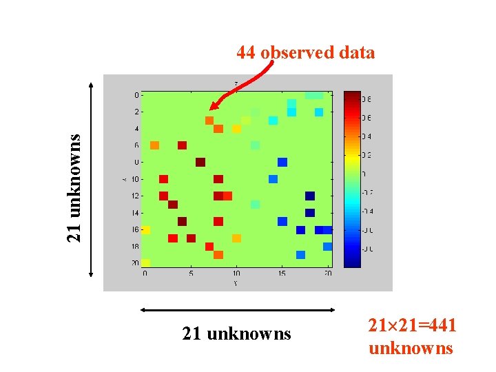
21 unknowns 44 observed data 21 unknowns 21 21=441 unknowns

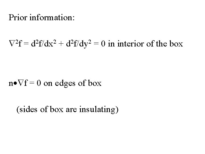
Prior information: 2 f = d 2 f/dx 2 + d 2 f/dy 2 = 0 in interior of the box n f = 0 on edges of box (sides of box are insulating)

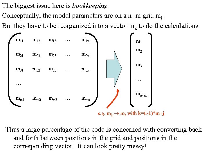
The biggest issue here is bookkeeping Conceptually, the model parameters are on a n m grid mij But they have to be reorganized into a vector mk to do the calculations m 11 m 12 m 13 … m 1 n m 21 m 22 m 23 … m 2 n m 31 m 32 m 33 … m 3 n m 2 m 3 … … mm 1 mm 2 mm 3 … mmn mn m e. g. mij mk with k=(i-1)*m+j Thus a large percentage of the code is concerned with converting back and forth between positions in the grid and positions in the corresponding vector. It can look pretty messy!

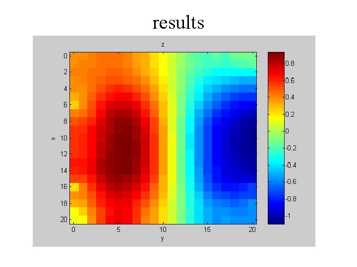
results

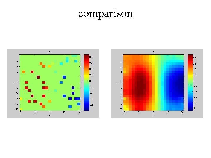
comparison

Example 3 Linear Systems

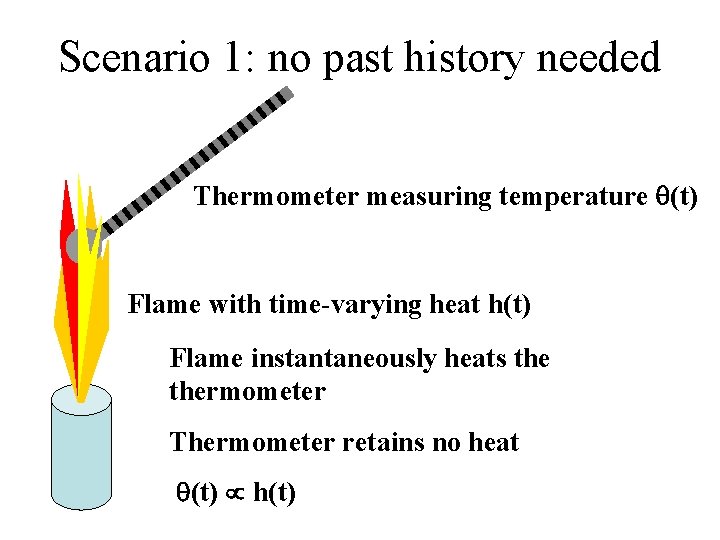
Scenario 1: no past history needed Thermometer measuring temperature q(t) Flame with time-varying heat h(t) Flame instantaneously heats thermometer Thermometer retains no heat q(t) h(t)

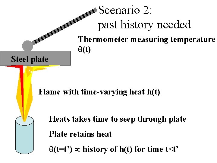
Scenario 2: past history needed Thermometer measuring temperature q(t) Steel plate Flame with time-varying heat h(t) Heats takes time to seep through plate Plate retains heat q(t=t’) history of h(t) for time t<t’

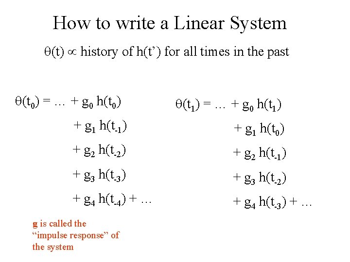
How to write a Linear System q(t) history of h(t’) for all times in the past q(t 0) = … + g 0 h(t 0) q(t 1) = … + g 0 h(t 1) + g 1 h(t-1) + g 1 h(t 0) + g 2 h(t-2) + g 2 h(t-1) + g 3 h(t-3) + g 3 h(t-2) + g 4 h(t-4) + … + g 4 h(t-3) + … g is called the “impulse response” of the system

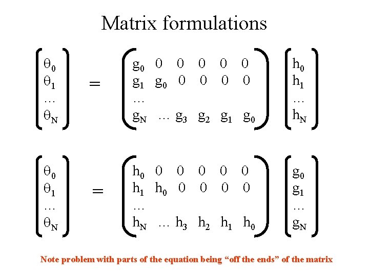
Matrix formulations q 0 q 1 … q. N = g 0 0 0 g 1 g 0 0 0 … g. N … g 3 g 2 g 1 g 0 h 1 … h. N = h 0 0 0 h 1 h 0 0 0 … h. N … h 3 h 2 h 1 h 0 g 1 … g. N Note problem with parts of the equation being “off the ends” of the matrix

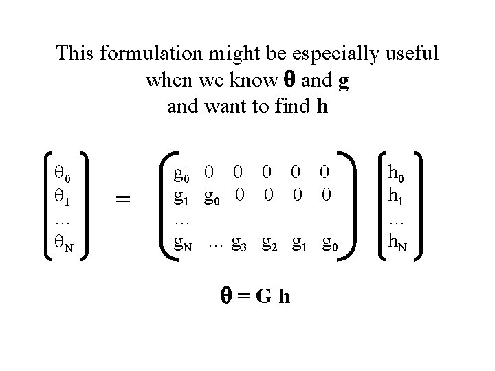
This formulation might be especially useful when we know q and g and want to find h q 0 q 1 … q. N = g 0 0 0 g 1 g 0 0 0 … g. N … g 3 g 2 g 1 g 0 q=Gh h 0 h 1 … h. N

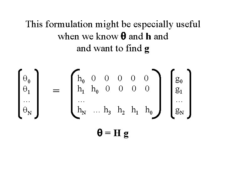
This formulation might be especially useful when we know q and h and want to find g q 0 q 1 … q. N = h 0 0 0 h 1 h 0 0 0 … h. N … h 3 h 2 h 1 h 0 q=Hg g 0 g 1 … g. N

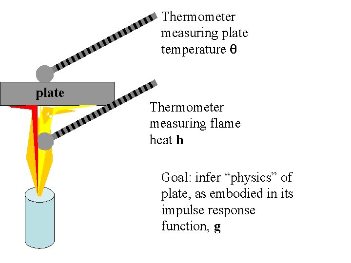
Thermometer measuring plate temperature q plate Thermometer measuring flame heat h Goal: infer “physics” of plate, as embodied in its impulse response function, g

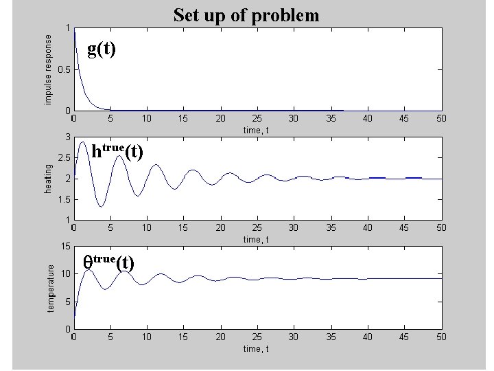
Set up of problem g(t) htrue(t) qtrue(t)

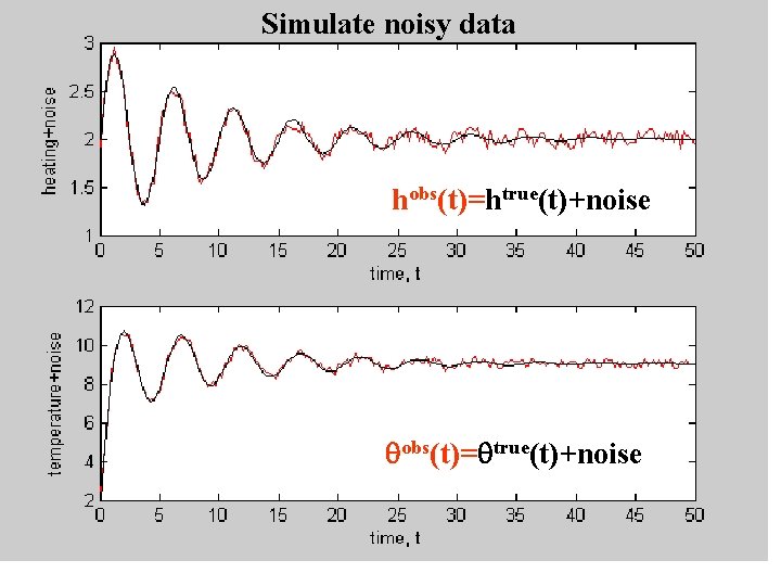
Simulate noisy data hobs(t)=htrue(t)+noise qobs(t)=qtrue(t)+noise

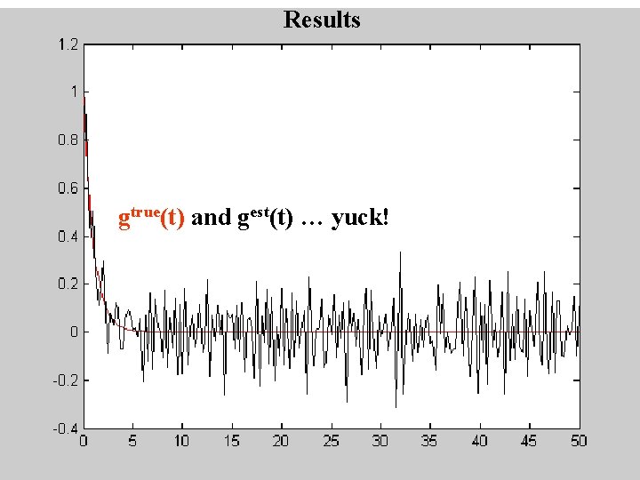
Results gtrue(t) and gest(t) … yuck!

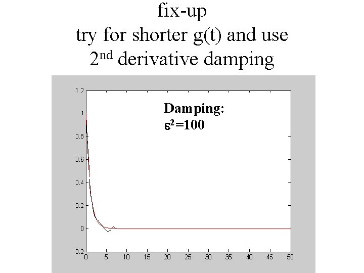
fix-up try for shorter g(t) and use 2 nd derivative damping Damping: e 2=100

Example 4 prediction error filter how well does the past predict the present?

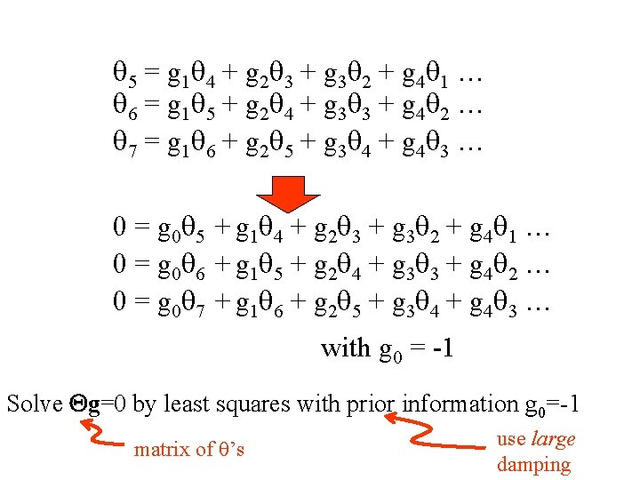
q 5 = g 1 q 4 + g 2 q 3 + g 3 q 2 + g 4 q 1 … q 6 = g 1 q 5 + g 2 q 4 + g 3 q 3 + g 4 q 2 … q 7 = g 1 q 6 + g 2 q 5 + g 3 q 4 + g 4 q 3 … 0 = g 0 q 5 + g 1 q 4 + g 2 q 3 + g 3 q 2 + g 4 q 1 … 0 = g 0 q 6 + g 1 q 5 + g 2 q 4 + g 3 q 3 + g 4 q 2 … 0 = g 0 q 7 + g 1 q 6 + g 2 q 5 + g 3 q 4 + g 4 q 3 … with g 0 = -1 Solve Qg=0 by least squares with prior information g 0=-1 matrix of q’s use large damping

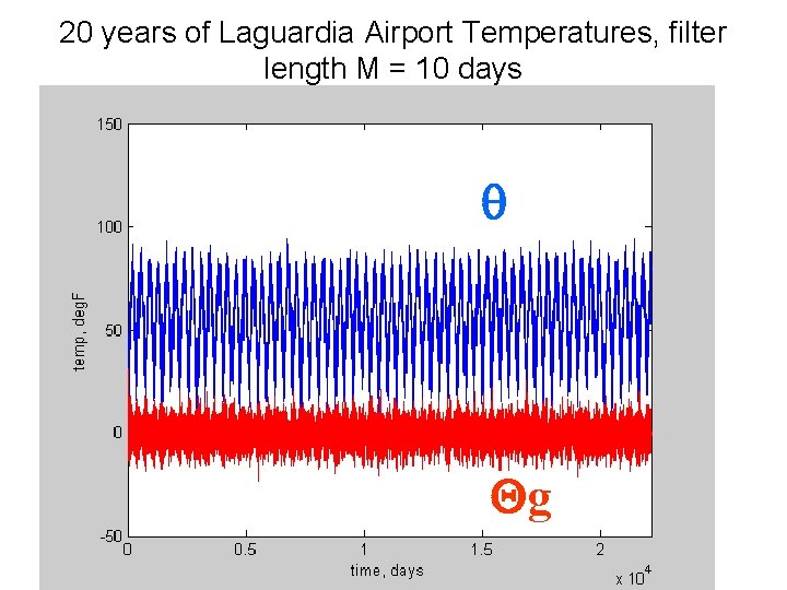
20 years of Laguardia Airport Temperatures, filter length M = 10 days q Qg

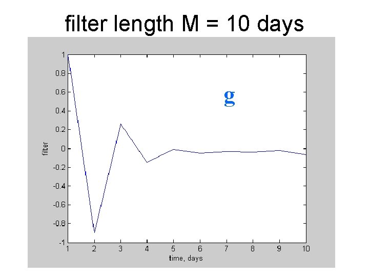
filter length M = 10 days g

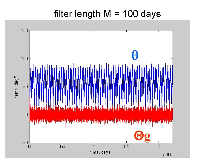
filter length M = 100 days q Qg

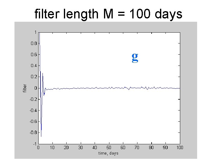
filter length M = 100 days g

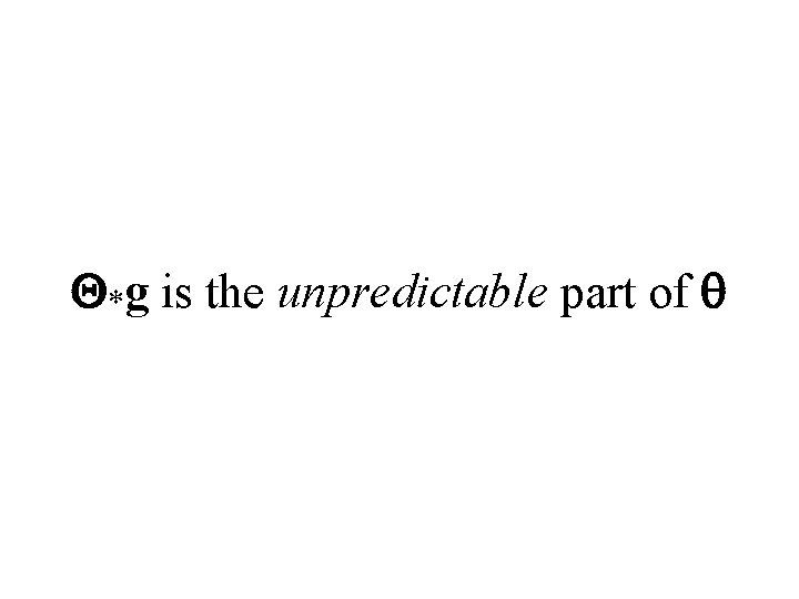
Q*g is the unpredictable part of q

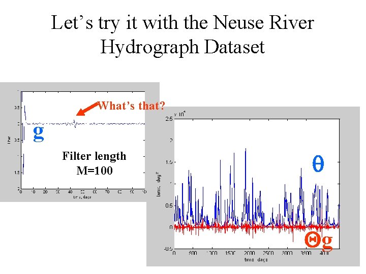
Let’s try it with the Neuse River Hydrograph Dataset What’s that? g Filter length M=100 q Qg

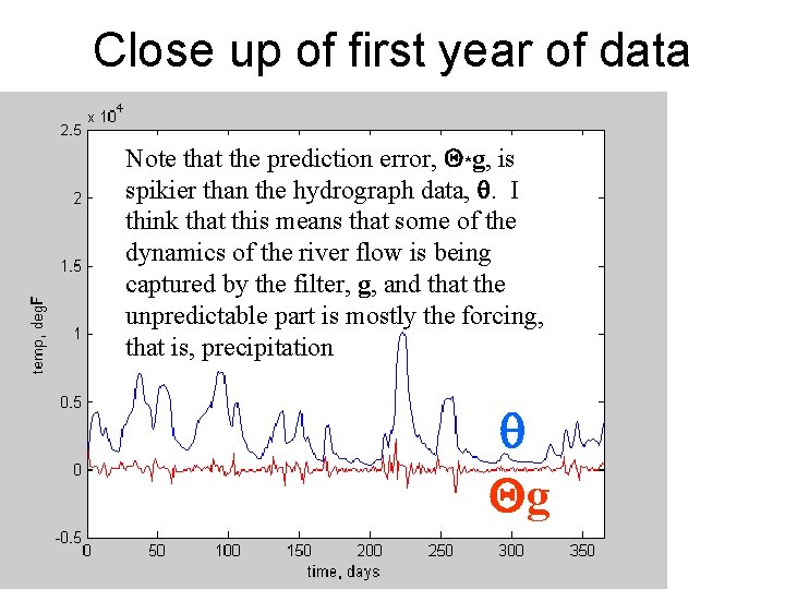
Close up of first year of data Note that the prediction error, Q*g, is spikier than the hydrograph data, q. I think that this means that some of the dynamics of the river flow is being captured by the filter, g, and that the unpredictable part is mostly the forcing, that is, precipitation q Qg

Example 4 Tomography

Tomography: reconstructing an image from measurements made along rays CAT scan: density image, reconstructed from X-ray absorption Seismic Tomography: velocity image, reconstructed from seismic ray travel times MRI : proton density image, reconstructed from radio wave emission intensity along lines of constant precession frequency

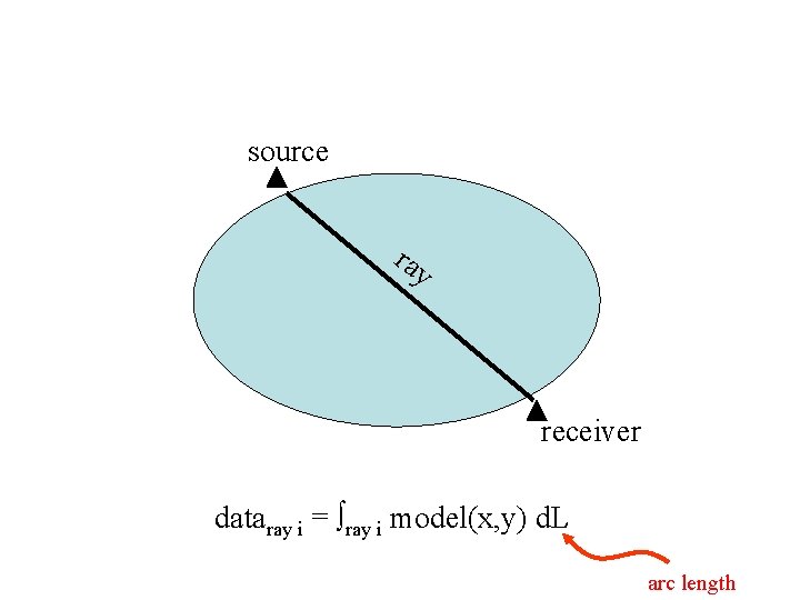
source ray receiver dataray i = ray i model(x, y) d. L arc length

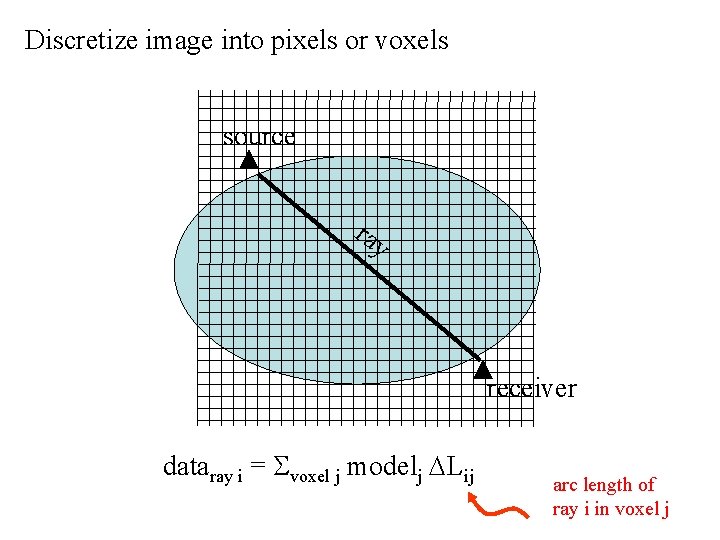
Discretize image into pixels or voxels source ray receiver dataray i = Svoxel j modelj DLij arc length of ray i in voxel j

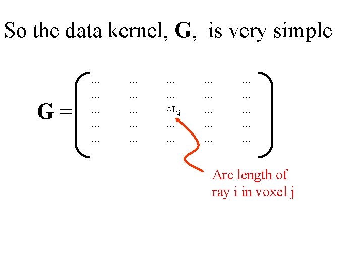
So the data kernel, G, is very simple G= … … … DLij … … … Arc length of ray i in voxel j

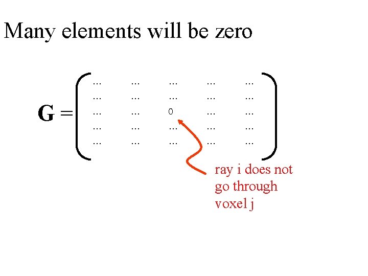
Many elements will be zero G= … … … 0 … … … ray i does not go through voxel j

the hard parts are: 1. computing the ray paths, if they are more complicated than straight lines 2. book-keeping, e. g. figuring out which rays pass through which voxels

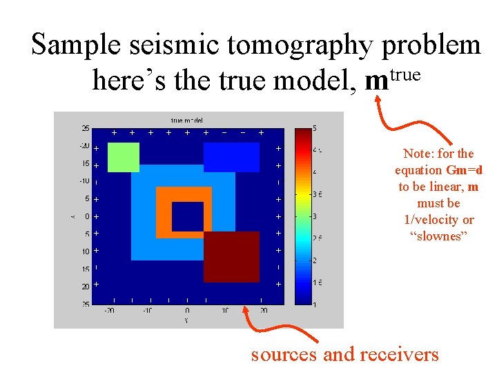
Sample seismic tomography problem here’s the true model, mtrue Note: for the equation Gm=d to be linear, m must be 1/velocity or “slownes” sources and receivers

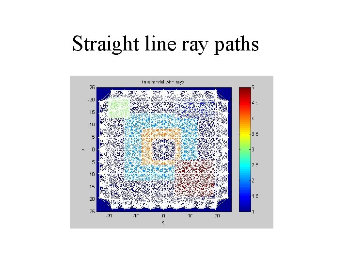
Straight line ray paths

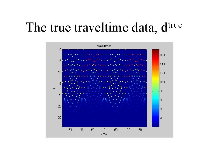
The true traveltime data, dtrue

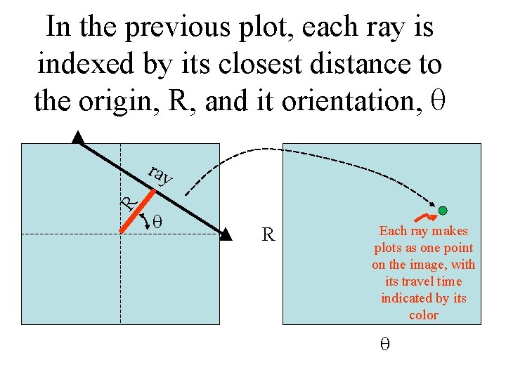
In the previous plot, each ray is indexed by its closest distance to the origin, R, and it orientation, q R ray q R Each ray makes plots as one point on the image, with its travel time indicated by its color q

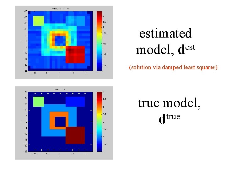
estimated est model, d (solution via damped least squares) true model, dtrue

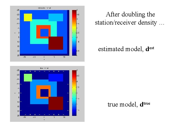
After doubling the station/receiver density … estimated model, dest true model, dtrue