LECTURE 4 NLPmodel for minimizing heat exchanger surface

LECTURE 4 • NLP-model for minimizing heat exchanger surface area costs • Simultaneous MINLP model

What did we learn in Lecture 3 • LP-model (either basic transshipment model or extended transshipment model) – Min. hot and cold utility consumption – Pinch point (and number of sub-networks) • MILP-model (extended transshipment model with binary variables for heat exchanger matches) – Min. number of heat exchangers – Matches (which streams exchange heat) – Head loads for all heat exchangers

What will we learn in Lecture 4 • Cost optimization of HENS (area minimization) with an NLP superstructure • Simultaneous MINLPmodel (Synheat-model) for – Min utilities – Min number of heat exchangers – Min HEX area

Heat exchanger network structure NLP-model minimising heat exchanger surface area costs

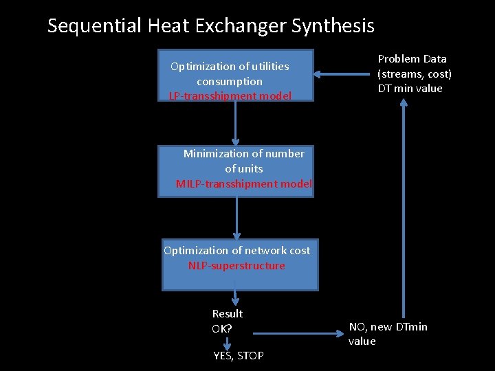
Sequential Heat Exchanger Synthesis Optimization of utilities consumption LP-transshipment model Problem Data (streams, cost) DT min value Minimization of number of units MILP-transshipment model Optimization of network cost NLP-superstructure Result OK? YES, STOP NO, new DTmin value

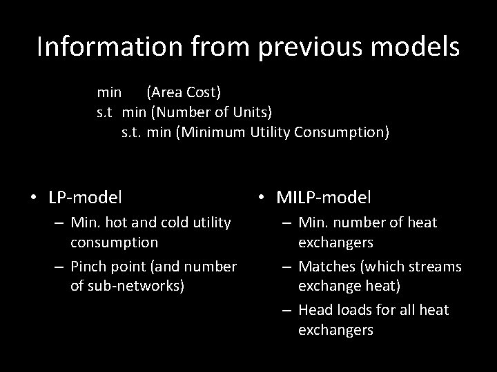
Information from previous models min (Area Cost) s. t min (Number of Units) s. t. min (Minimum Utility Consumption) • LP-model – Min. hot and cold utility consumption – Pinch point (and number of sub-networks) • MILP-model – Min. number of heat exchangers – Matches (which streams exchange heat) – Head loads for all heat exchangers

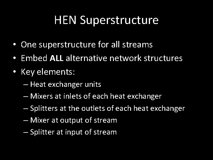
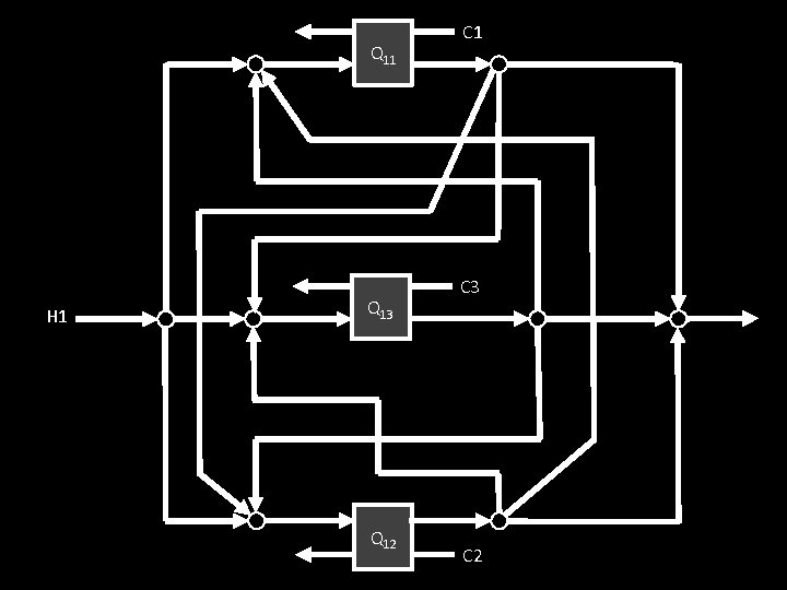
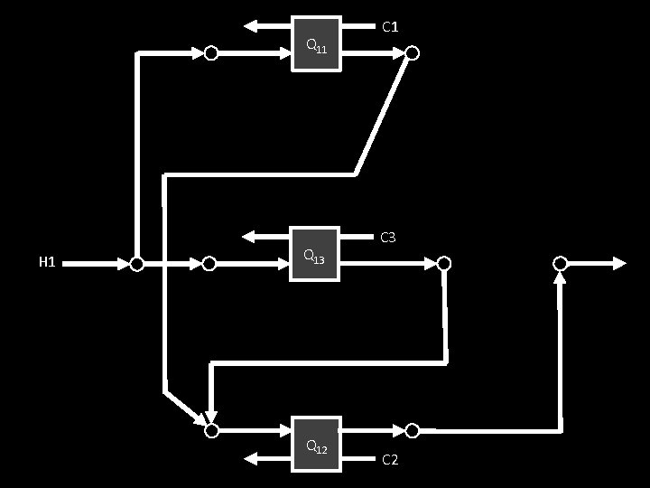
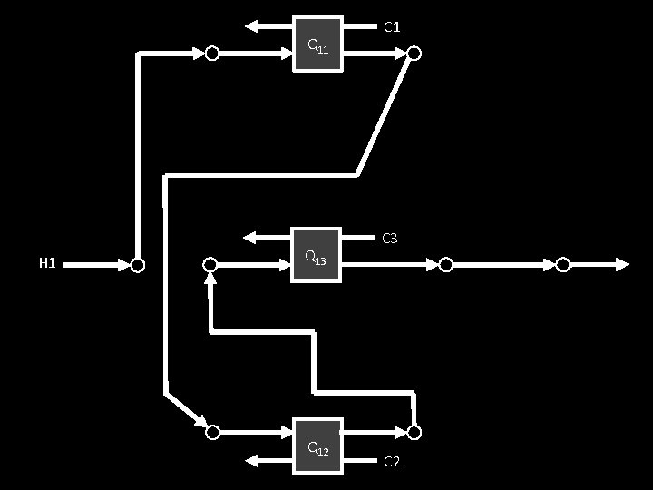
HEN Superstructure • One superstructure for all streams • Embed ALL alternative network structures • Key elements: – Heat exchanger units – Mixers at inlets of each heat exchanger – Splitters at the outlets of each heat exchanger – Mixer at output of stream – Splitter at input of stream

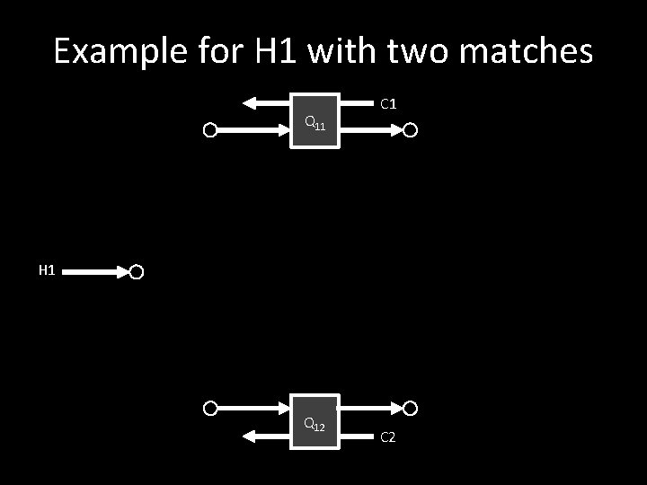
Example for H 1 with two matches Q 11 C 1 H 1 Q 12 C 2

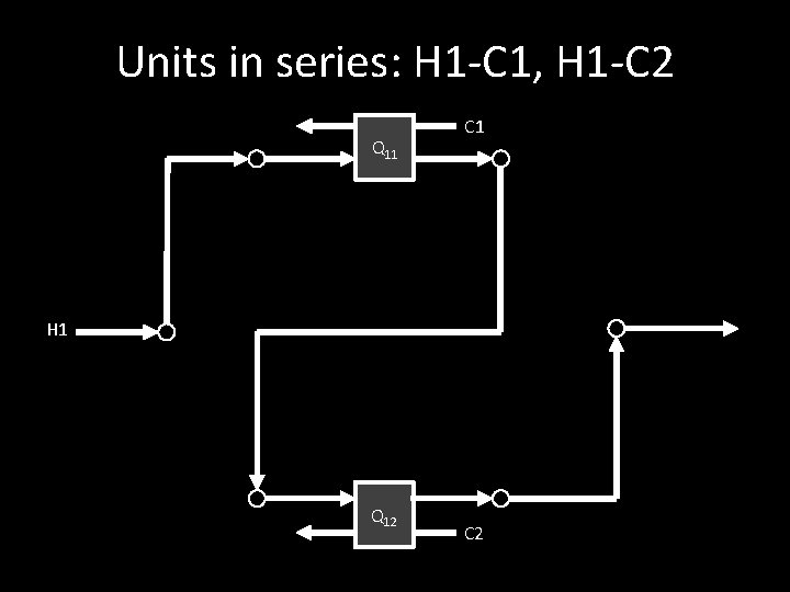
Units in series: H 1 -C 1, H 1 -C 2 Q 11 C 1 H 1 Q 12 C 2

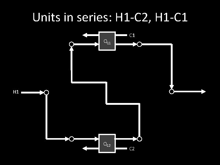
Units in series: H 1 -C 2, H 1 -C 1 Q 11 C 1 H 1 Q 12 C 2

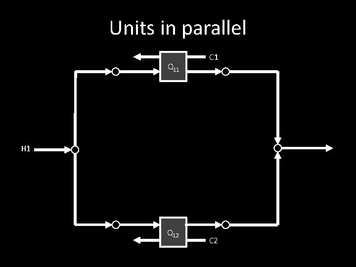
Units in parallel Q 11 C 1 H 1 Q 12 C 2

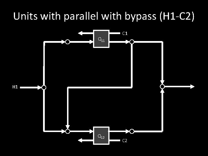
Units with parallel with bypass (H 1 -C 2) Q 11 C 1 H 1 Q 12 C 2

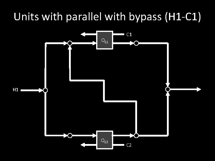
Units with parallel with bypass (H 1 -C 1) Q 11 C 1 H 1 Q 12 C 2

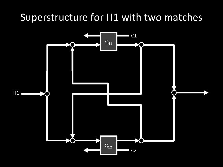
Superstructure for H 1 with two matches Q 11 C 1 H 1 Q 12 C 2

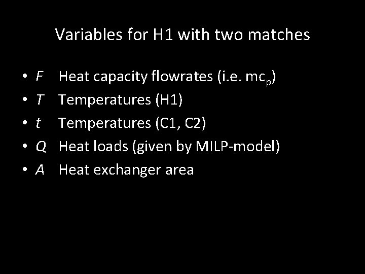
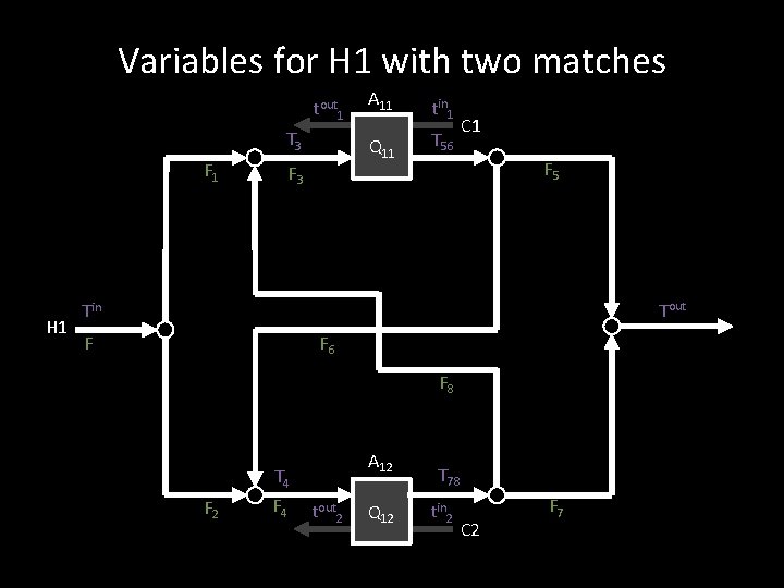
Variables for H 1 with two matches • • • F T t Q A Heat capacity flowrates (i. e. mcp) Temperatures (H 1) Temperatures (C 1, C 2) Heat loads (given by MILP-model) Heat exchanger area

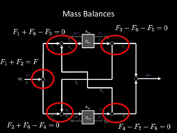
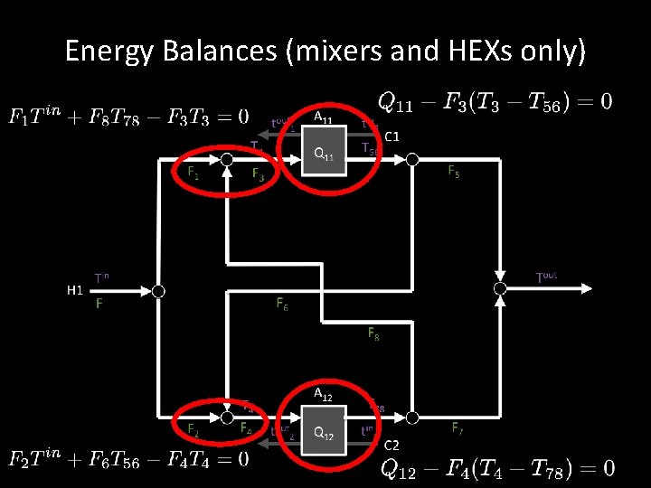
Variables for H 1 with two matches tout 1 T 3 F 1 H 1 F 3 A 11 tin 1 Q 11 T 56 C 1 F 5 Tout Tin F 6 F F 8 F 2 T 4 F 4 A 12 tout 2 Q 12 T 78 tin 2 C 2 F 7

Mass Balances

Energy Balances (mixers and HEXs only)

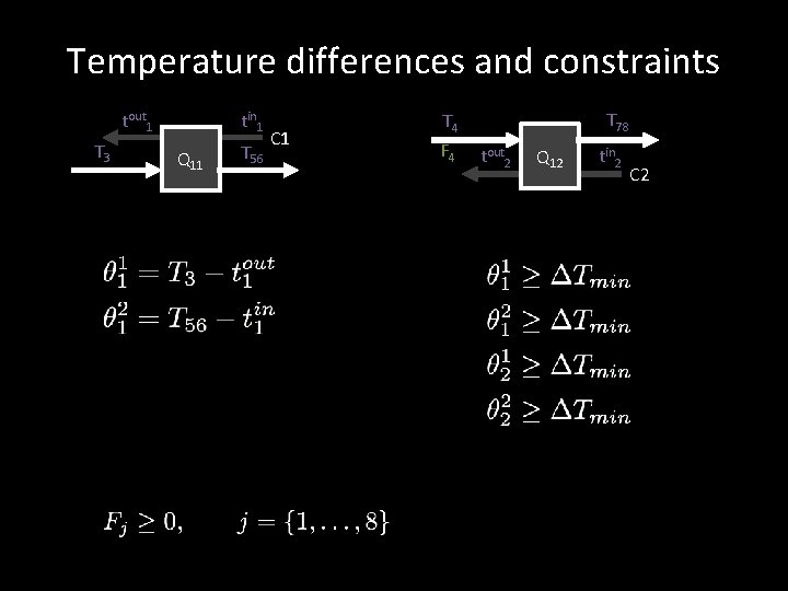
Temperature differences and constraints tin 1 tout 1 T 3 Q 11 T 56 C 1 T 4 F 4 T 78 tout 2 Q 12 tin 2 C 2

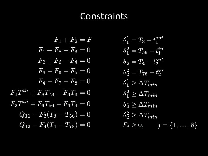
Constraints

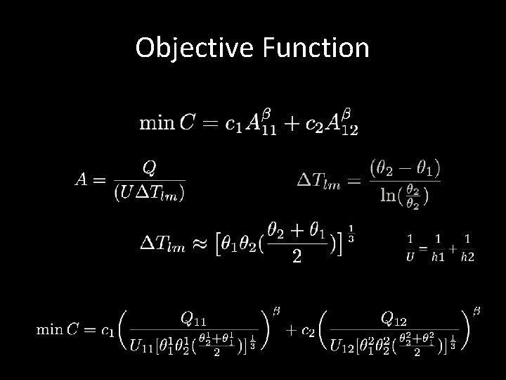
Objective Function

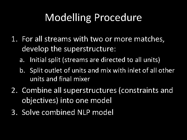
Modelling Procedure 1. For all streams with two or more matches, develop the superstructure: a. Initial split (streams are directed to all units) b. Split outlet of units and mix with inlet of all other units and final mixer 2. Combine all superstructures (constraints and objectives) into one model 3. Solve combined NLP model

Q 11 H 1 Q 13 Q 12 C 1 C 3 C 2

Q 11 H 1 Q 13 Q 12 C 1 C 3 C 2

Q 11 H 1 Q 13 Q 12 C 1 C 3 C 2

Sequential Heat Exchanger Synthesis Optimization of utilities consumption LP-transshipment model Problem Data (streams, cost) DT min value Minimization of number of units MILP-transshipment model Optimization of network cost NLP-superstructure Result OK? YES, STOP NO, new DTmin value

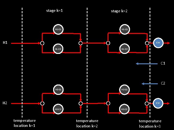
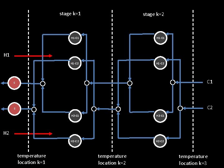
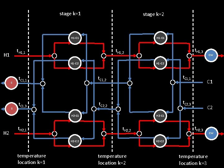
Simultaneous MINLP model Synheat, stagewise superstructure

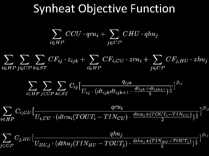
Optimisation Problem min Total Cost = Area Cost + Units Fixed Cost + Utility Cost

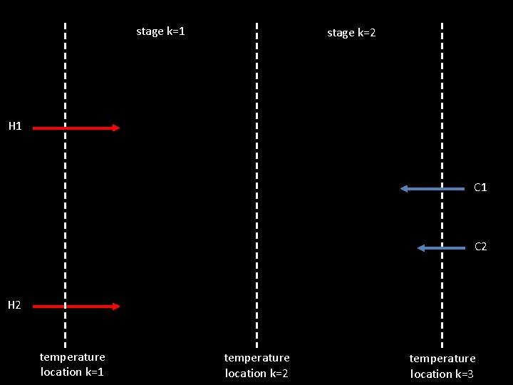
stage k=1 stage k=2 H 1 C 2 H 2 temperature location k=1 temperature location k=2 temperature location k=3

stage k=1 stage k=2 H 1 -C 1 H 1 CW H 1 -C 2 C 1 C 2 H 2 -C 1 H 2 CW H 2 -C 2 temperature location k=1 H 2 -C 2 temperature location k=3

stage k=1 stage k=2 H 1 -C 1 H 1 -C 2 H 1 S C 2 H 2 -C 1 H 2 -C 2 H 2 temperature location k=1 temperature location k=2 temperature location k=3

stage k=1 stage k=2 H 1 -C 1 t. H 1, 1 H 1 S t. C 1, 1 t. C 1, 2 t. C 1, 1 t. C 1, 3 t. C 2, 2 t. C 2, 3 H 2 -C 1 H 2 t. H 2, 1 C 2 H 2 -C 1 t. H 2, 3 t. H 2, 2 H 2 -C 2 temperature location k=1 CW H 1 -C 2 S t. H 1, 3 t. H 1, 2 H 2 -C 2 temperature location k=3 CW

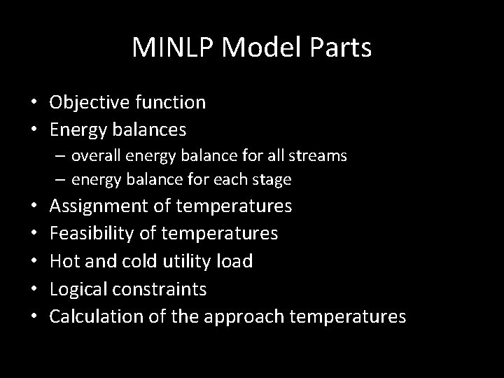
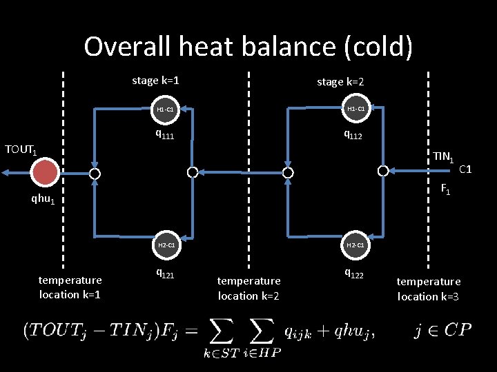
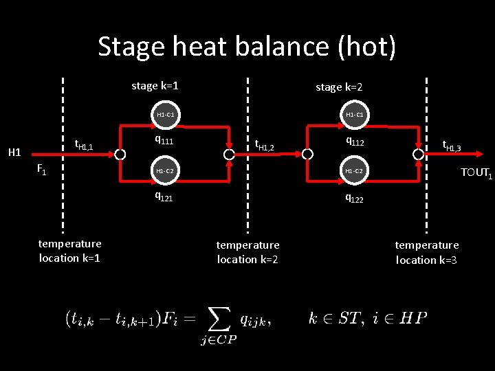
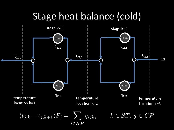
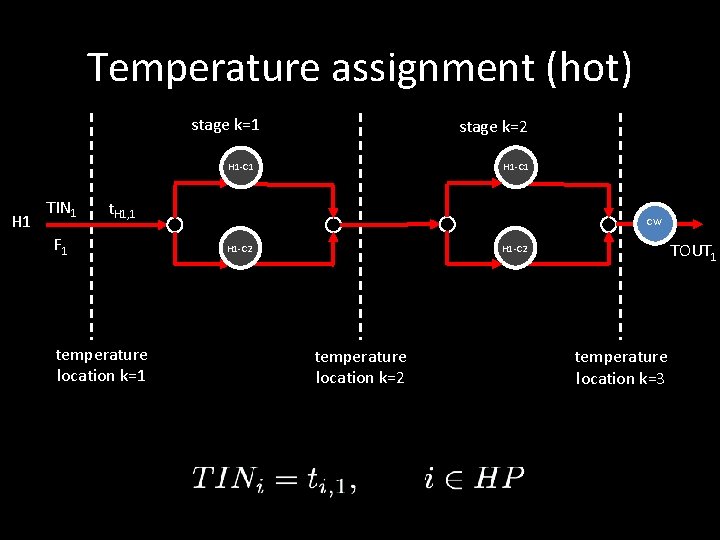
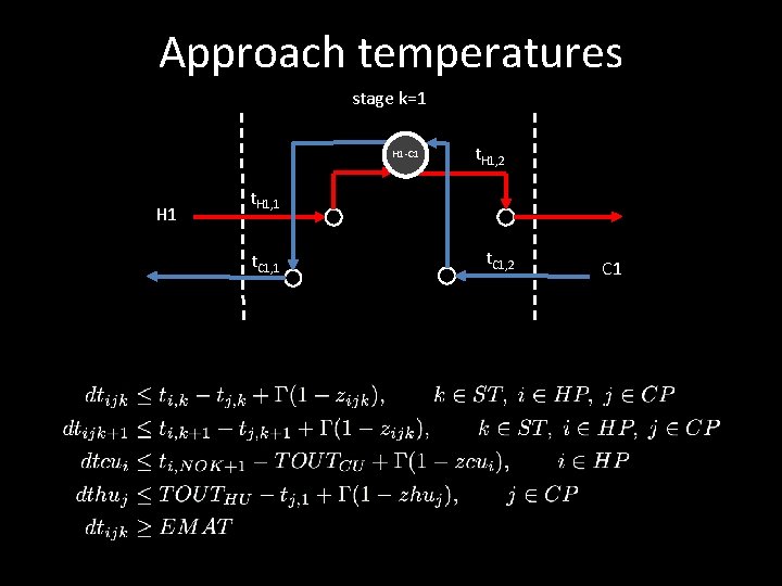
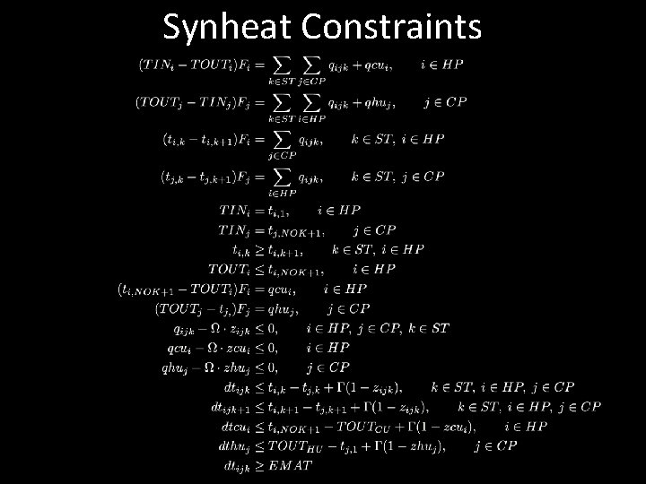
MINLP Model Parts • Objective function • Energy balances – overall energy balance for all streams – energy balance for each stage • • • Assignment of temperatures Feasibility of temperatures Hot and cold utility load Logical constraints Calculation of the approach temperatures

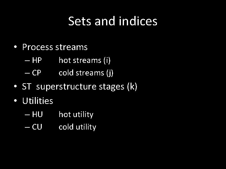
Sets and indices • Process streams – HP – CP hot streams (i) cold streams (j) • ST superstructure stages (k) • Utilities – HU – CU hot utility cold utility

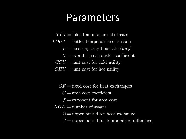
Parameters

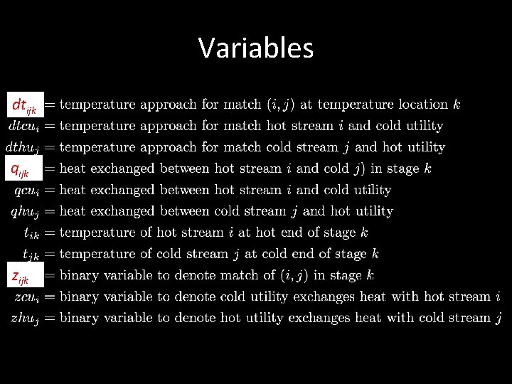
Variables dtijk qijk zijk

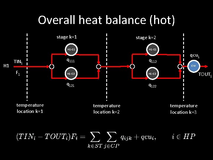
Overall heat balance (hot) stage k=1 stage k=2 H 1 -C 1 H 1 TIN 1 F 1 temperature location k=1 q 112 H 1 -C 2 q 121 q 122 temperature location k=2 qcu 1 CW TOUT 1 temperature location k=3

Overall heat balance (cold) stage k=1 stage k=2 H 1 -C 1 q 111 TOUT 1 q 112 TIN 1 S F 1 qhu 1 temperature location k=1 C 1 H 2 -C 1 q 122 temperature location k=3

Stage heat balance (hot) stage k=1 stage k=2 H 1 -C 1 t. H 1, 1 H 1 F 1 temperature location k=1 q 111 t. H 1, 2 q 112 H 1 -C 2 q 121 q 122 temperature location k=2 t. H 1, 3 TOUT 1 temperature location k=3

Stage heat balance (cold) stage k=1 stage k=2 H 1 -C 1 q 111 t. C 1, 3 t. C 1, 2 t. C 1, 1 temperature location k=1 q 112 H 2 -C 1 q 121 q 122 temperature location k=2 C 1 temperature location k=3

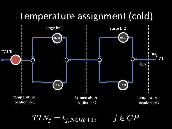
Temperature assignment (hot) stage k=1 stage k=2 H 1 -C 1 H 1 TIN 1 t. H 1, 1 F 1 temperature location k=1 CW TOUT 1 H 1 -C 2 temperature location k=2 temperature location k=3

Temperature assignment (cold) stage k=1 stage k=2 H 1 -C 1 TOUT 1 TIN 1 S t. C 1, 3 H 2 -C 1 temperature location k=1 C 1 H 2 -C 1 temperature location k=2 temperature location k=3

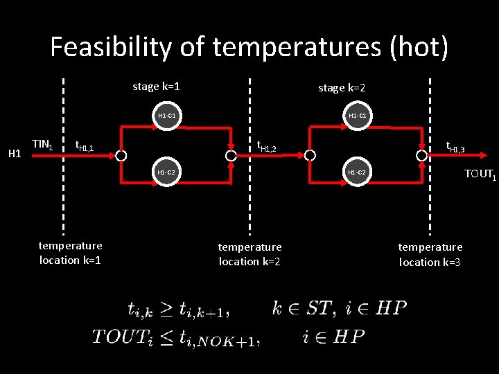
Feasibility of temperatures (hot) stage k=1 stage k=2 H 1 -C 1 H 1 TIN 1 t. H 1, 2 TOUT 1 H 1 -C 2 temperature location k=1 t. H 1, 3 temperature location k=2 temperature location k=3

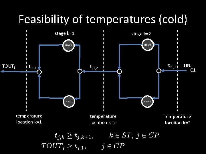
Feasibility of temperatures (cold) stage k=1 stage k=2 H 1 -C 1 TOUT 1 H 2 -C 1 temperature location k=1 t. C 1, 3 t. C 1, 2 t. C 1, 1 TIN 1 C 1 H 2 -C 1 temperature location k=2 temperature location k=3

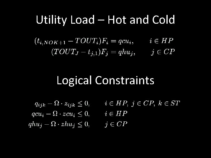
Utility Load – Hot and Cold Logical Constraints

Approach temperatures stage k=1 H 1 -C 1 H 1 t. H 1, 2 t. H 1, 1 t. C 1, 2 C 1

Synheat Constraints

Synheat Objective Function

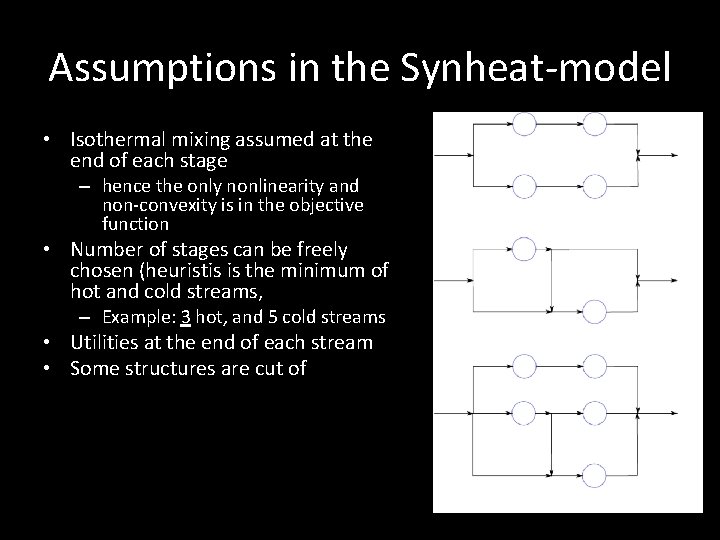
Assumptions in the Synheat-model • Isothermal mixing assumed at the end of each stage – hence the only nonlinearity and non-convexity is in the objective function • Number of stages can be freely chosen (heuristis is the minimum of hot and cold streams, – Example: 3 hot, and 5 cold streams • Utilities at the end of each stream • Some structures are cut of

Sequential vs. simultaneous • The submodels in the sequential approach are easier to solve (more robust and less-time consuming) – MILP-step is still NP-hard (nonpolynomial) • The decomposition into the sequential steps can cut of the best solution – If global optimization algorithms are used, simultaneous approaches can find the global optimum for the original problem