Lecture 4 Linear Regression Analysis Steps in Data

Lecture 4 – Linear Regression Analysis

Steps in Data Analysis Step 1: Collect and clean data (spreadsheet from heaven) Step 2: Calculate descriptive statistics Step 3: Explore graphics Step 4: Choose outcome(s) and potential predictive variables (covariates) Step 5: Pick an appropriate statistical procedure & execute Step 6: Evaluate fitted model, make adjustments as needed

Choice of Analysis Four Considerations 1) Purpose of the investigation Descriptive orientation 2) The mathematical characteristics of the variables Level of measurement (nominal, ordinal, continuous) and Distribution 3) The statistical assumptions made about these variables Distribution, Independence, etc. 4) How the data are collected Random sample, cohort, case control, etc.

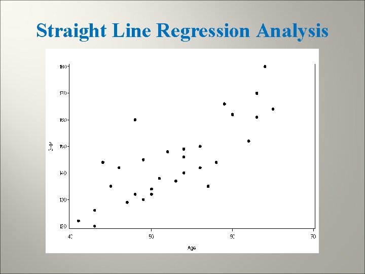
Simple Linear Regression Purpose of analysis: To relate two variables, where we designate one as the outcome of interest (Dependent Variable or DV) and one more as the predictor variables (Independent Variables or IVs) In general, we will consider k to represent the number of IVs and here k=1. Given a sample of n individuals, we observe pairs of values for 2 variables (Xi, Yi) for each individual i. Type of variables: Continuous (interval or ratio)

Straight Line Regression Analysis

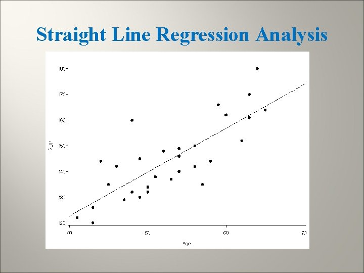
Straight Line Regression Analysis

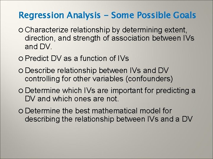
Regression Analysis - Some Possible Goals Characterize relationship by determining extent, direction, and strength of association between IVs and DV. Predict DV as a function of IVs Describe relationship between IVs and DV controlling for other variables (confounders) Determine which IVs are important for predicting a DV and which ones are not. Determine the best mathematical model for describing the relationship between IVs and a DV

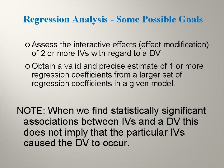
Regression Analysis - Some Possible Goals Assess the interactive effects (effect modification) of 2 or more IVs with regard to a DV Obtain a valid and precise estimate of 1 or more regression coefficients from a larger set of regression coefficients in a given model. NOTE: When we find statistically significant associations between IVs and a DV this does not imply that the particular IVs caused the DV to occur.

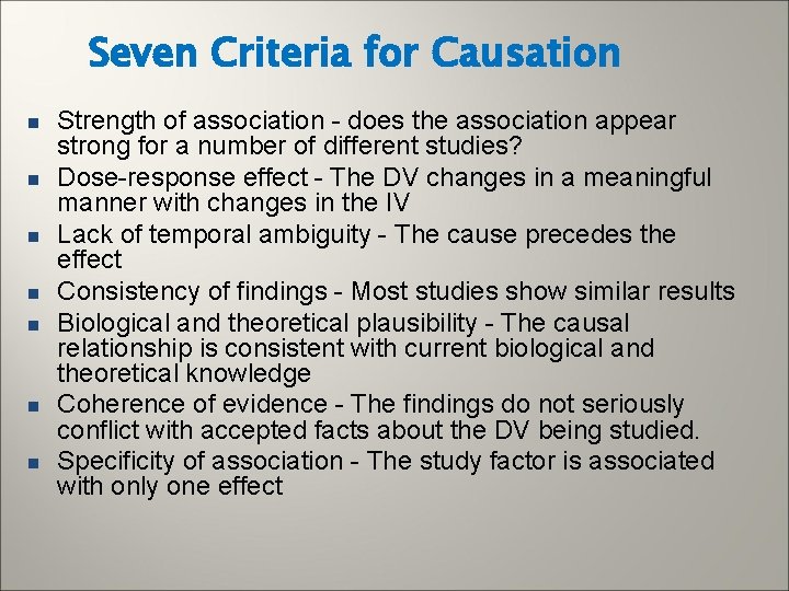
Seven Criteria for Causation n n n Strength of association - does the association appear strong for a number of different studies? Dose-response effect - The DV changes in a meaningful manner with changes in the IV Lack of temporal ambiguity - The cause precedes the effect Consistency of findings - Most studies show similar results Biological and theoretical plausibility - The causal relationship is consistent with current biological and theoretical knowledge Coherence of evidence - The findings do not seriously conflict with accepted facts about the DV being studied. Specificity of association - The study factor is associated with only one effect

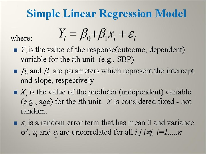
Simple Linear Regression Model where: n Yi is the value of the response(outcome, dependent) variable for the ith unit (e. g. , SBP) n 0 and 1 are parameters which represent the intercept and slope, respectively n Xi is the value of the predictor (independent) variable (e. g. , age) for the ith unit. X is considered fixed - not random. n i is a random error term that has mean 0 and variance 2, i and j are uncorrelated for all i, j i j, i=1, . . . , n

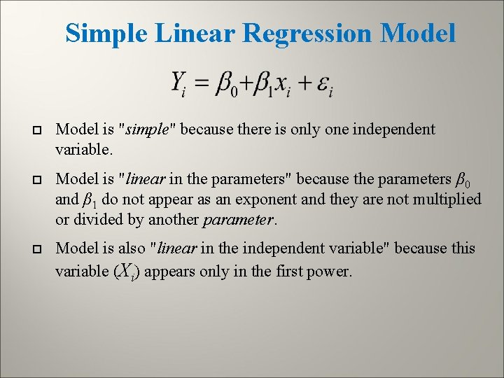
Simple Linear Regression Model is "simple" because there is only one independent variable. Model is "linear in the parameters" because the parameters β 0 and β 1 do not appear as an exponent and they are not multiplied or divided by another parameter. Model is also "linear in the independent variable" because this variable (Xi) appears only in the first power.

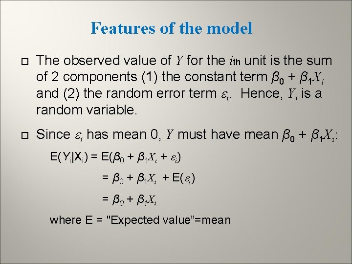
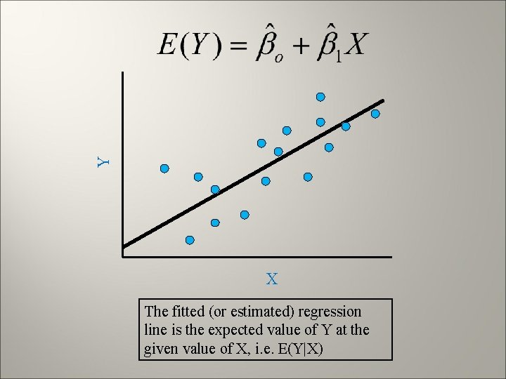
Features of the model The observed value of Y for the ith unit is the sum of 2 components (1) the constant term β 0 + β 1 Xi and (2) the random error term i. Hence, Yi is a random variable. Since i has mean 0, Y must have mean β 0 + β 1 Xi: E(Yi|Xi) = E(β 0 + β 1 Xi + i) = β 0 + β 1 Xi + E( i) = β 0 + β 1 X i where E = "Expected value”=mean

Y X The fitted (or estimated) regression line is the expected value of Y at the given value of X, i. e. E(Y|X)

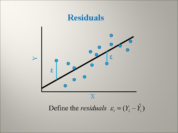
Residuals Y ε ε X

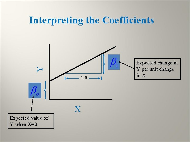
Y Interpreting the Coefficients 1. 0 X Expected value of Y when X=0 Expected change in Y per unit change in X

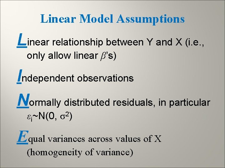
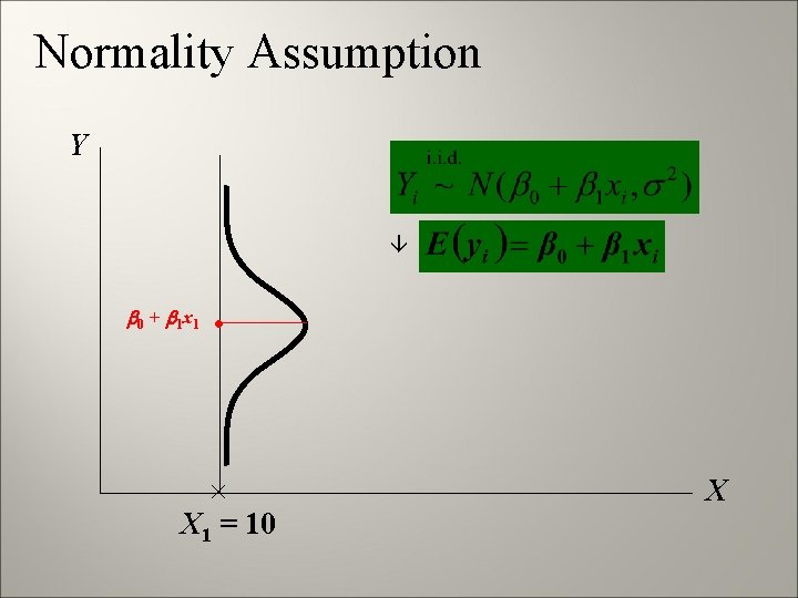
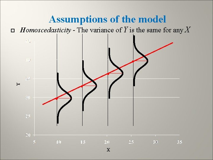
Linear Model Assumptions Linear relationship between Y and X (i. e. , only allow linear β’s) Independent observations Normally distributed residuals, in particular εi~N(0, σ2) Equal variances across values of X (homogeneity of variance)

Normality Assumption Y 0 + 1 x 1 • X 1 = 10 X

Assumptions of the model Homoscedasticity - The variance of Y is the same for any X • • • Y • X

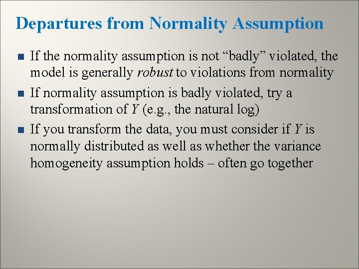
Departures from Normality Assumption n If the normality assumption is not “badly” violated, the model is generally robust to violations from normality If normality assumption is badly violated, try a transformation of Y (e. g. , the natural log) If you transform the data, you must consider if Y is normally distributed as well as whether the variance homogeneity assumption holds – often go together

Other Assumptions § The “correct” model is fitted All IVs included are truly related to the DV No (conceivable) IVs related to the DV have been left out Violation of either of these assumptions can lead to “model misspecification bias”

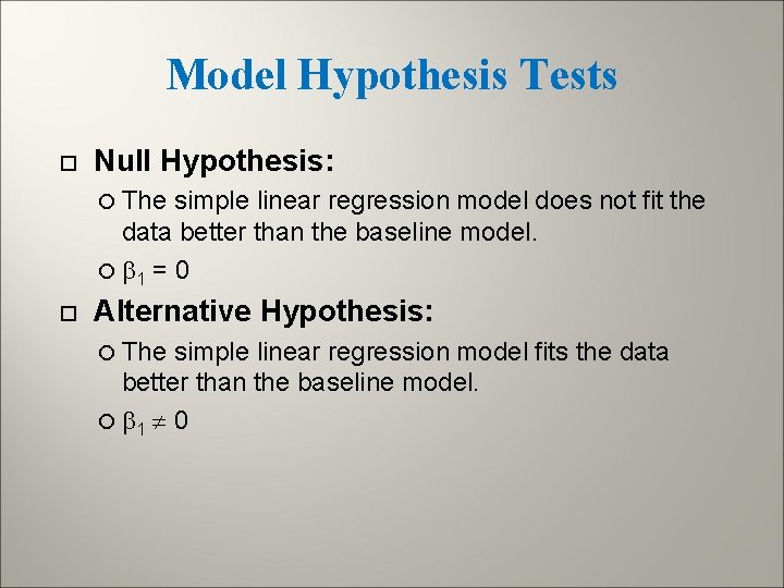
Model Hypothesis Tests Null Hypothesis: The simple linear regression model does not fit the data better than the baseline model. 1 = 0 Alternative Hypothesis: The simple linear regression model fits the data better than the baseline model. 1 0

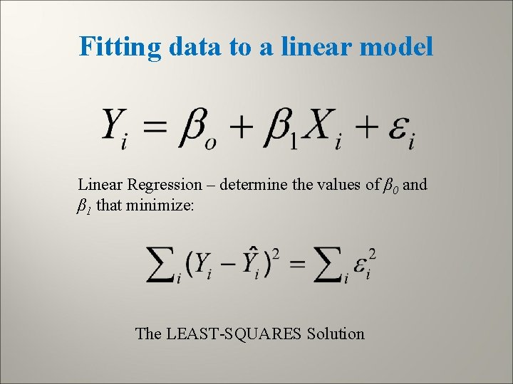
Fitting data to a linear model Linear Regression – determine the values of β 0 and β 1 that minimize: The LEAST-SQUARES Solution

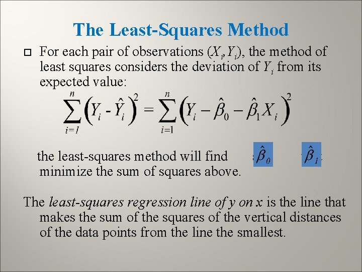
The Least-Squares Method For each pair of observations (Xi, Yi), the method of least squares considers the deviation of Yi from its expected value: the least-squares method will find and that minimize the sum of squares above. The least-squares regression line of y on x is the line that makes the sum of the squares of the vertical distances of the data points from the line the smallest.

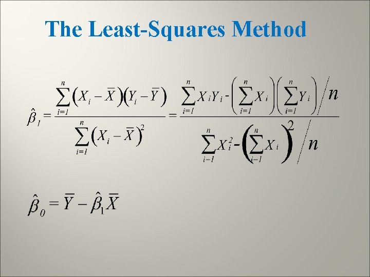
The Least-Squares Method

The Least Squares Method The method of least squares is purely mathematical However, statistically the least squares estimators are very appealing because the are the Best Linear Unbiased Estimators (BLUE) This means that among all of the equations we could have picked to estimate 0 and 1, the least squares equations will give us estimates: 1. That have expectation 0 and 1 (unbiased) 2. Have minimum variance among all of the possible linear estimators for 0 and 1 (most efficient)

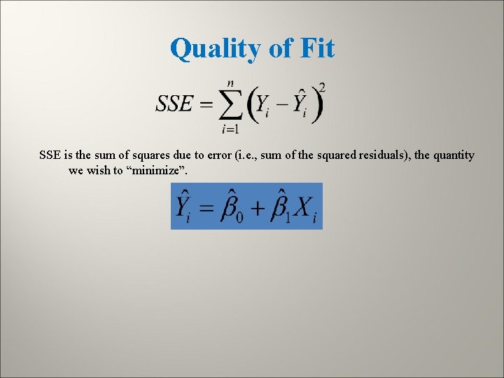
Quality of Fit SSE is the sum of squares due to error (i. e. , sum of the squared residuals), the quantity we wish to “minimize”.

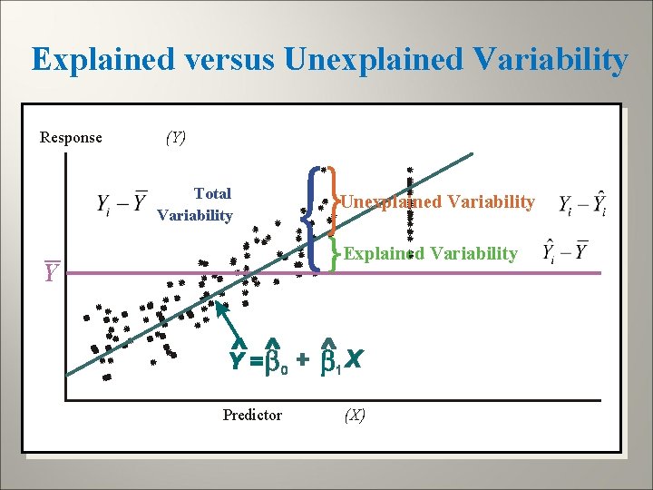
Explained versus Unexplained Variability Response (Y) Total Variability _ Unexplained Variability Explained Variability Y Predictor (X)

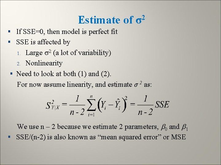
Estimate of σ2 § If SSE=0, then model is perfect fit § SSE is affected by Large 2 (a lot of variability) 2. Nonlinearity § Need to look at both (1) and (2). For now assume linearity, and estimate σ 2 as: 1. We use n – 2 because we estimate 2 parameters, 0 and 1 § SSE/(n-2) is also known as “mean squared error” or MSE

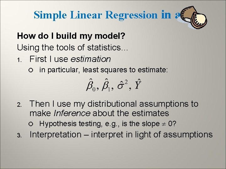
Simple Linear Regression in a How do I build my model? Using the tools of statistics… 1. First I use estimation 2. Then I use my distributional assumptions to make Inference about the estimates 3. in particular, least squares to estimate: Hypothesis testing, e. g. , is the slope 0? Interpretation – interpret in light of assumptions

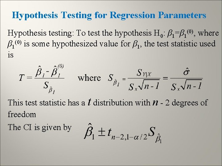
Hypothesis Testing for Regression Parameters Hypothesis testing: To test the hypothesis H 0: β 1=β 1(0), where β 1(0) is some hypothesized value for β 1, the test statistic used is This test statistic has a t distribution with n - 2 degrees of freedom The CI is given by

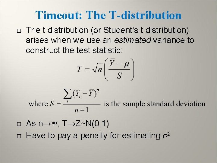
Timeout: The T-distribution The t distribution (or Student’s t distribution) arises when we use an estimated variance to construct the test statistic: As n→∞, T→Z~N(0, 1) Have to pay a penalty for estimating σ2

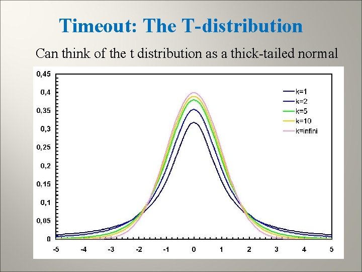
Timeout: The T-distribution Can think of the t distribution as a thick-tailed normal

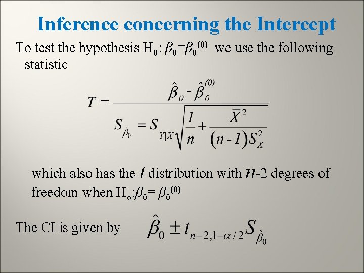
Inference concerning the Intercept To test the hypothesis H 0: β 0=β 0(0) we use the following statistic which also has the t distribution with n-2 degrees of freedom when Ho: β 0= β 0(0) The CI is given by

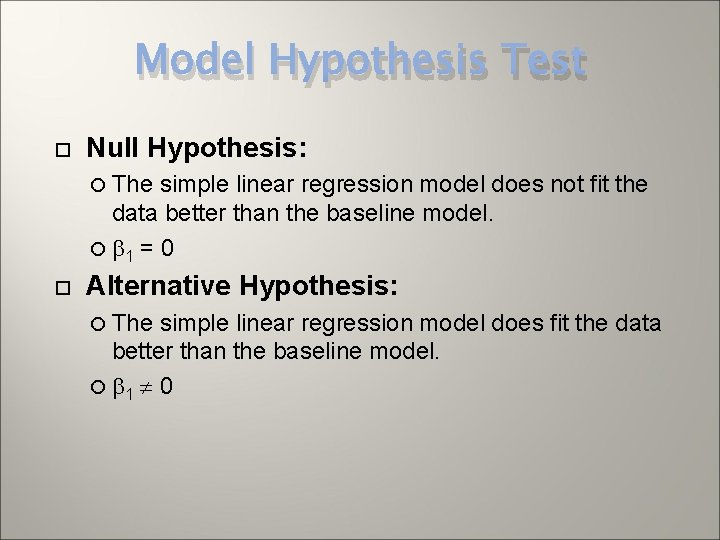
Model Hypothesis Test Null Hypothesis: The simple linear regression model does not fit the data better than the baseline model. 1 = 0 Alternative Hypothesis: The simple linear regression model does fit the data better than the baseline model. 1 0

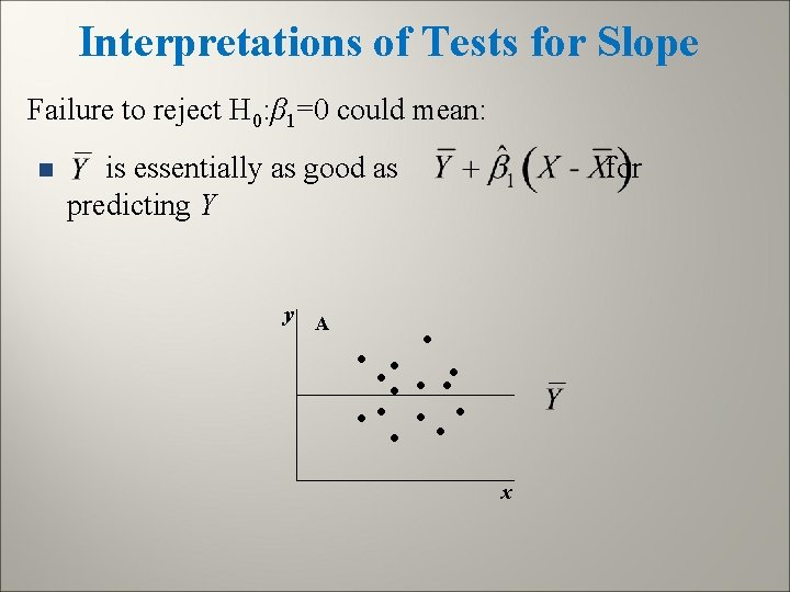
Interpretations of Tests for Slope Failure to reject H 0: β 1=0 could mean: n is essentially as good as for predicting Y y A • • • • • x

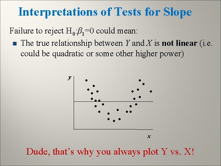
Interpretations of Tests for Slope Failure to reject H 0: β 1=0 could mean: n The true relationship between Y and X is not linear (i. e. could be quadratic or some other higher power) y • • • • • • • • • x Dude, that’s why you always plot Y vs. X!

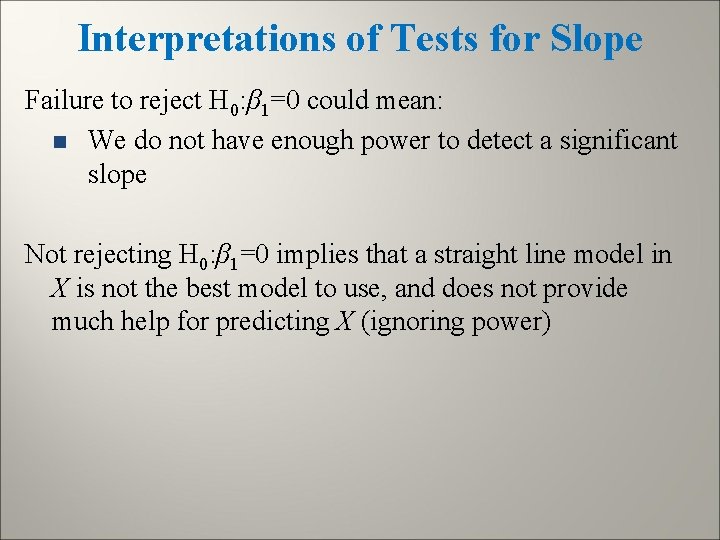
Interpretations of Tests for Slope Failure to reject H 0: β 1=0 could mean: n We do not have enough power to detect a significant slope Not rejecting H 0: β 1=0 implies that a straight line model in X is not the best model to use, and does not provide much help for predicting X (ignoring power)

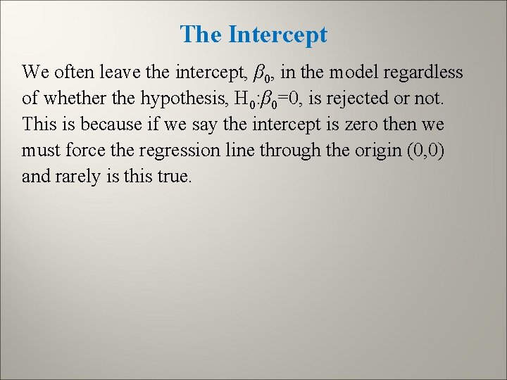
The Intercept We often leave the intercept, β 0, in the model regardless of whether the hypothesis, H 0: β 0=0, is rejected or not. This is because if we say the intercept is zero then we must force the regression line through the origin (0, 0) and rarely is this true.

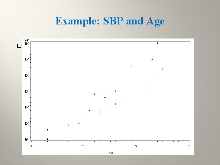
Example: SBP and Age Regression of SBP on age:

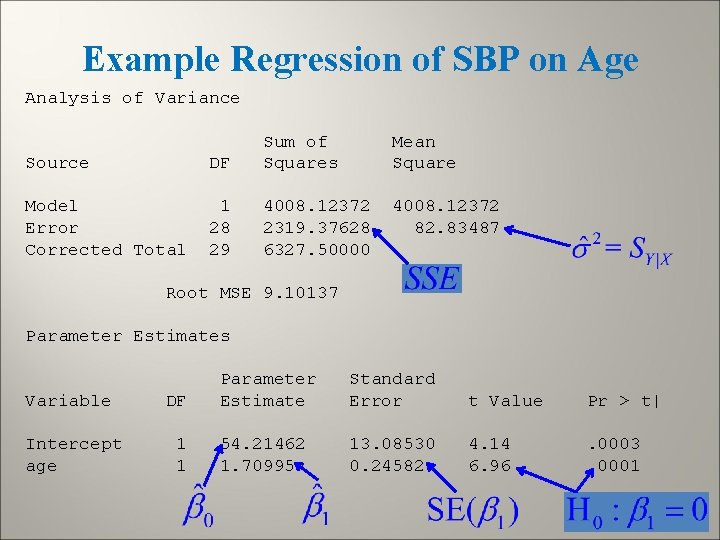
Example Regression of SBP on Age Analysis of Variance Source DF Sum of Squares Model Error Corrected Total 1 28 29 4008. 12372 2319. 37628 6327. 50000 Mean Square 4008. 12372 82. 83487 Root MSE 9. 10137 Parameter Estimates Variable Intercept age DF 1 1 Parameter Estimate Standard Error t Value Pr > t| 54. 21462 1. 70995 13. 08530 0. 24582 4. 14 6. 96 . 0003. 0001

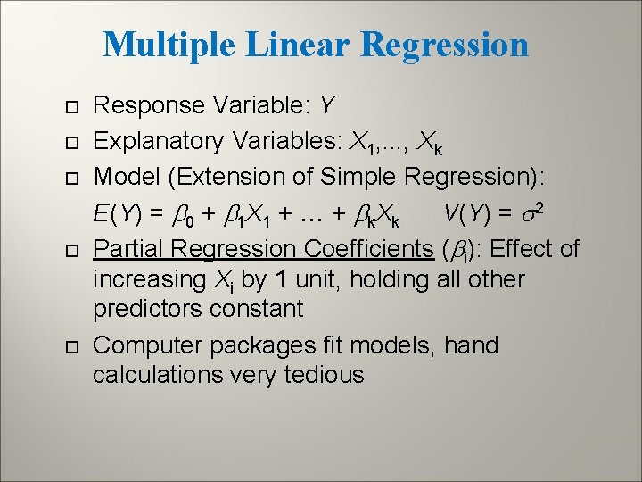
Multiple Linear Regression Response Variable: Y Explanatory Variables: X 1, . . . , Xk Model (Extension of Simple Regression): E(Y) = 0 + 1 X 1 + + k. Xk V(Y) = s 2 Partial Regression Coefficients ( i): Effect of increasing Xi by 1 unit, holding all other predictors constant Computer packages fit models, hand calculations very tedious

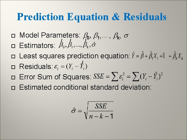
Prediction Equation & Residuals Model Parameters: 0, 1, …, k, s Estimators: Least squares prediction equation: Residuals: Error Sum of Squares: Estimated conditional standard deviation:

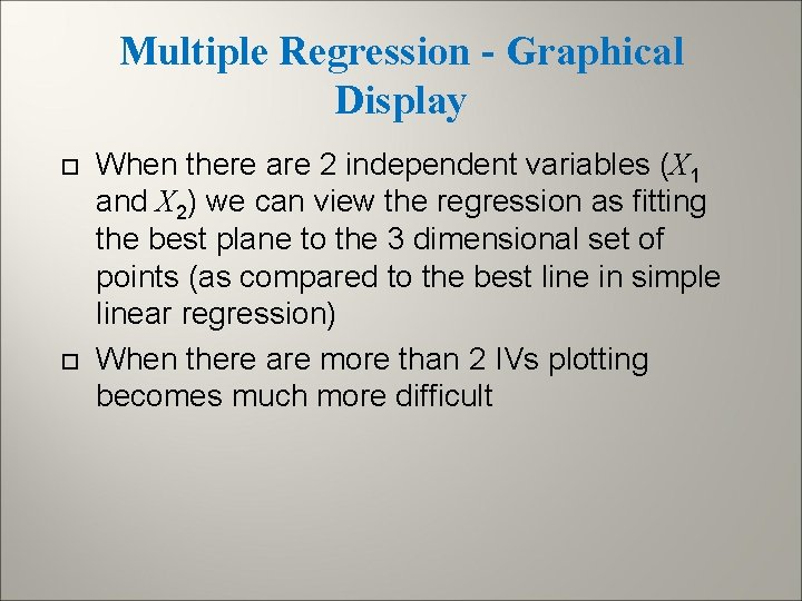
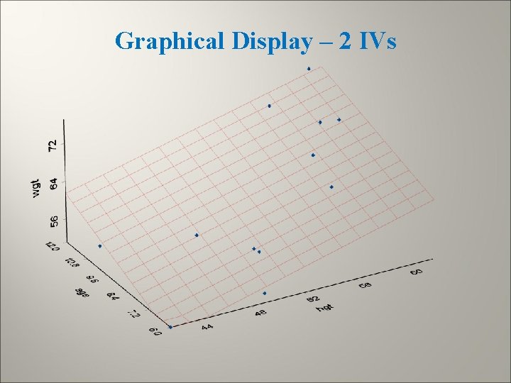
Multiple Regression - Graphical Display When there are 2 independent variables (X 1 and X 2) we can view the regression as fitting the best plane to the 3 dimensional set of points (as compared to the best line in simple linear regression) When there are more than 2 IVs plotting becomes much more difficult

Graphical Display – 2 IVs

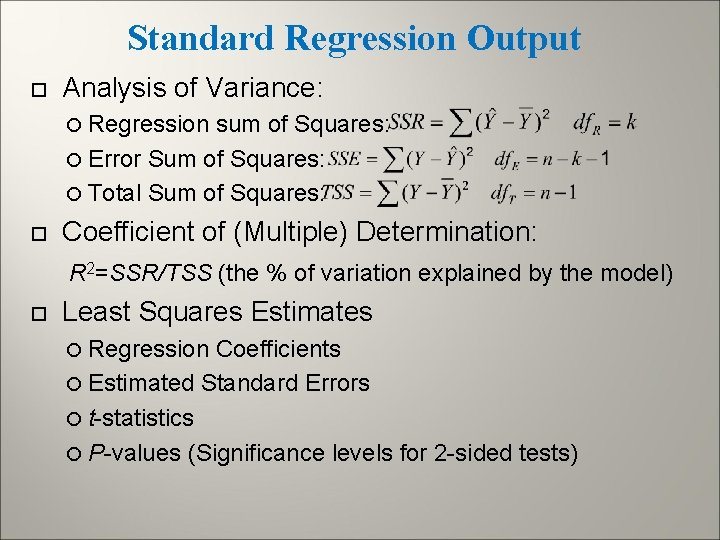
Standard Regression Output Analysis of Variance: Regression sum of Squares: Error Sum of Squares: Total Sum of Squares: Coefficient of (Multiple) Determination: R 2=SSR/TSS (the % of variation explained by the model) Least Squares Estimates Regression Coefficients Estimated Standard Errors t-statistics P-values (Significance levels for 2 -sided tests)

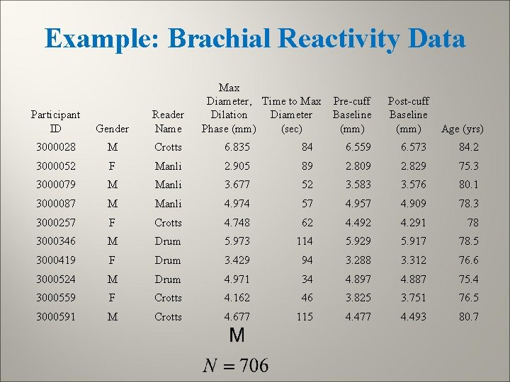
Example: Brachial Reactivity Data Max Diameter, Time to Max Pre-cuff Dilation Diameter Baseline Phase (mm) (sec) (mm) Post-cuff Baseline (mm) Age (yrs) Participant ID Gender Reader Name 3000028 M Crotts 6. 835 84 6. 559 6. 573 84. 2 3000052 F Manli 2. 905 89 2. 809 2. 829 75. 3 3000079 M Manli 3. 677 52 3. 583 3. 576 80. 1 3000087 M Manli 4. 974 57 4. 909 78. 3 3000257 F Crotts 4. 748 62 4. 492 4. 291 78 3000346 M Drum 5. 973 114 5. 929 5. 917 78. 5 3000419 F Drum 3. 429 94 3. 288 3. 312 76. 6 3000524 M Drum 4. 971 34 4. 897 4. 887 75. 4 3000559 F Crotts 4. 162 46 3. 825 3. 751 76. 5 3000591 M Crotts 4. 677 115 4. 477 4. 493 80. 7

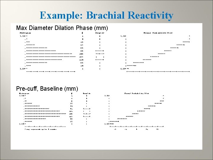
Example: Brachial Reactivity Max Diameter Dilation Phase (mm) Histogram 7. 75+*. *. ***********************************************. **** 2. 25+* ----+----+----+----+ # 1 4 12 27 65 96 146 157 114 65 14 1 Boxplot 0 0 | | | +-----+ *--+--* | | +-----+ | | | Normal Probability Plot 7. 75+ * | *****+ | ******+ | ******* | ***** |******++ 2. 25+*+ +----+----+----+----+----+ Pre-cuff, Baseline (mm) Histogram 7. 75+*. *. **********************************************. ******* 2. 25+* ----+----+----+----+---* may represent up to 4 counts # 1 3 6 25 54 91 131 156 132 80 25 2 Boxplot 0 0 0 | | +-----+ | | *--+--* +-----+ | | | Normal Probability Plot 7. 75+ * | ******+ | *****+ | +****** | ******* |****+ 2. 25+*+++ +----+----+----+----+----+ -2 -1 0 +1 +2

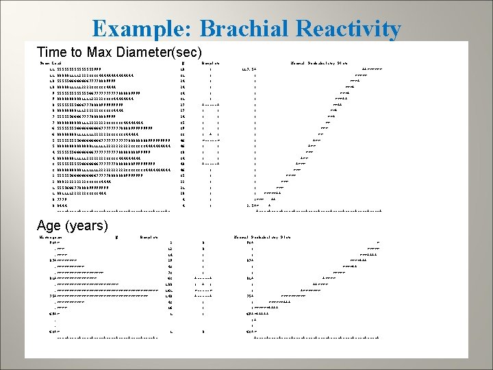
Example: Brachial Reactivity Time to Max Diameter(sec) Stem Leaf 11 55555555999 11 000001111222233334444444 10 55555666677778889999 10 000001111122223333334444 9 55555556677777888889999 9 0000011112222233334444 8 5555666777888899999 8 00001112222223333334444 7 555555666677778888889999 7 00000111222222233333334444 6 5555666667777888899999 6 00001111111222222333333344444 5 5555566666777777888899999 5 00000001111112222233333344444 4 5555555666677777888899999 4 00000001111122223333344444 3 5555566666667777777888888899999 3 000001111111222222333344444 2 555555666667777788888889999999 2 000222223333334444 1 55556667788889999 1 00111122222233333444 0 7779 0 0444 ----+----+----+----+----+- # 18 31 24 24 34 31 27 27 24 35 39 33 46 46 38 34 40 46 35 22 21 20 4 4 Boxplot | | | +-----+ | | | | | + | *-----* | | | +-----+ | | | | Normal Probability Plot 117. 5+ ++****** | ***+ | ***++ | **+ | ** | +** | *** | +*** | *** | *****++ |*** ++ 2. 5+* + +----+----+----+----+----+ Age (years) Histogram # Boxplot 93+*. **** 87+*********** 81+************************* 75+*******************. **** 69+*. . 63+* ----+----+----+----+- 2 12 14 29 43 73 63 100 161 148 43 16 1 1 0 0 | | +-----+ | *-----* +-----+ | | | 0 Normal Probability Plot 93+ * | ***** | ***++++ 87+ ****+++ | ***** 81+ +**** | +******* 75+ ***** | ******+++ |******++++ 69+*+++++ |+ | 63+* +----+----+----+----+----+

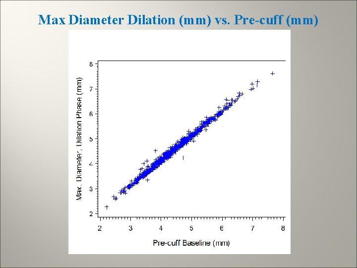
Max Diameter Dilation (mm) vs. Pre-cuff (mm)

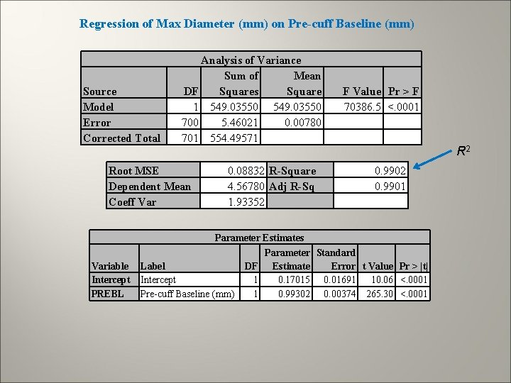
Regression of Max Diameter (mm) on Pre-cuff Baseline (mm) Source Model Error Corrected Total Analysis of Variance Sum of Mean DF Squares Square 1 549. 03550 700 5. 46021 0. 00780 701 554. 49571 Root MSE Dependent Mean Coeff Variable Intercept PREBL 0. 08832 R-Square 4. 56780 Adj R-Sq 1. 93352 F Value Pr > F 70386. 5 <. 0001 R 2 0. 9901 Parameter Estimates Parameter Standard Label DF Estimate Error t Value Pr > |t| Intercept 1 0. 17015 0. 01691 10. 06 <. 0001 Pre-cuff Baseline (mm) 1 0. 99302 0. 00374 265. 30 <. 0001

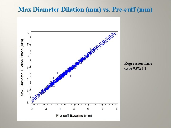
Max Diameter Dilation (mm) vs. Pre-cuff (mm) Regression Line with 95% CI

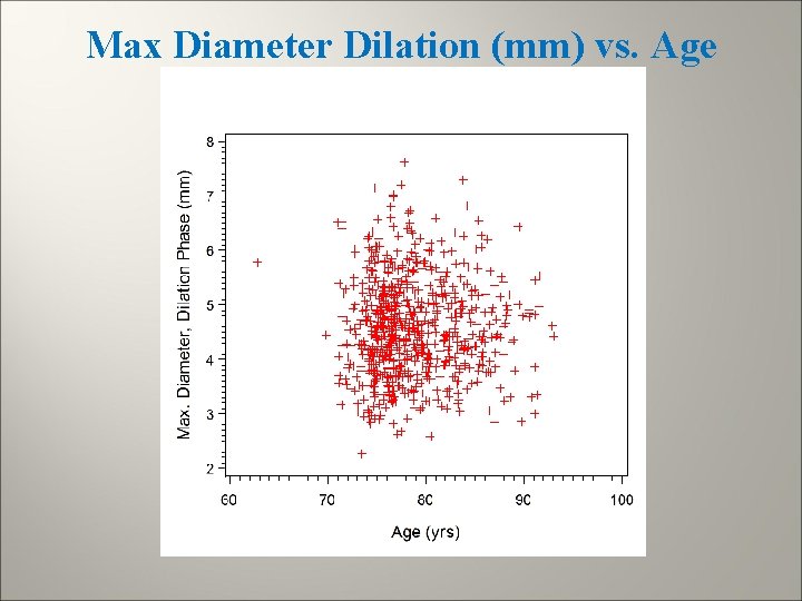
Max Diameter Dilation (mm) vs. Age

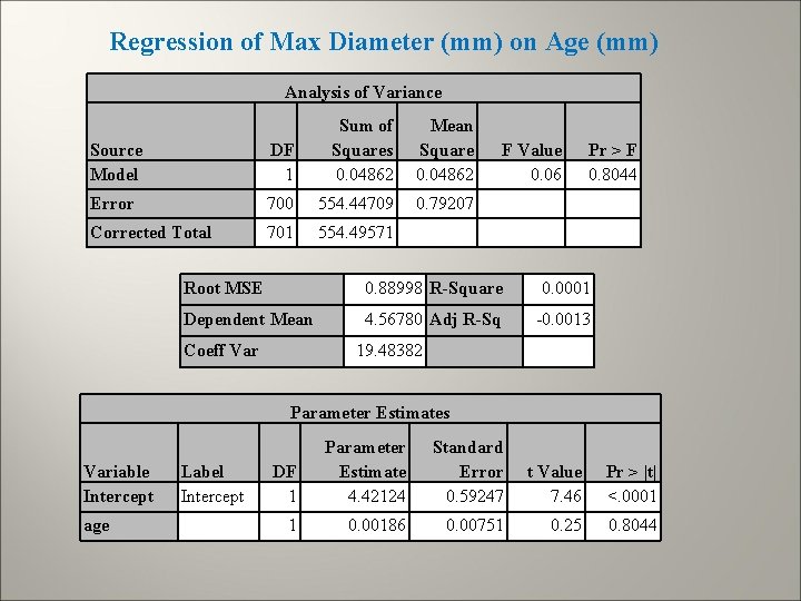
Regression of Max Diameter (mm) on Age (mm) Analysis of Variance Source Model DF 1 Sum of Squares 0. 04862 Error 700 554. 44709 Corrected Total 701 554. 49571 Mean Square 0. 04862 0. 79207 F Value 0. 06 Pr > F 0. 8044 Root MSE 0. 88998 R-Square 0. 0001 Dependent Mean 4. 56780 Adj R-Sq -0. 0013 Coeff Var 19. 48382 Parameter Estimates Variable Intercept age Label Intercept DF 1 Parameter Estimate 4. 42124 Standard Error 0. 59247 t Value 7. 46 Pr > |t| <. 0001 1 0. 00186 0. 00751 0. 25 0. 8044

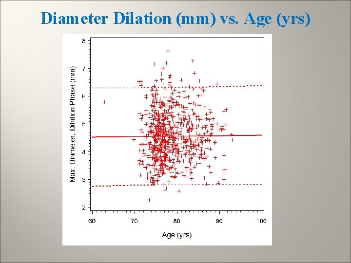
Diameter Dilation (mm) vs. Age (yrs)

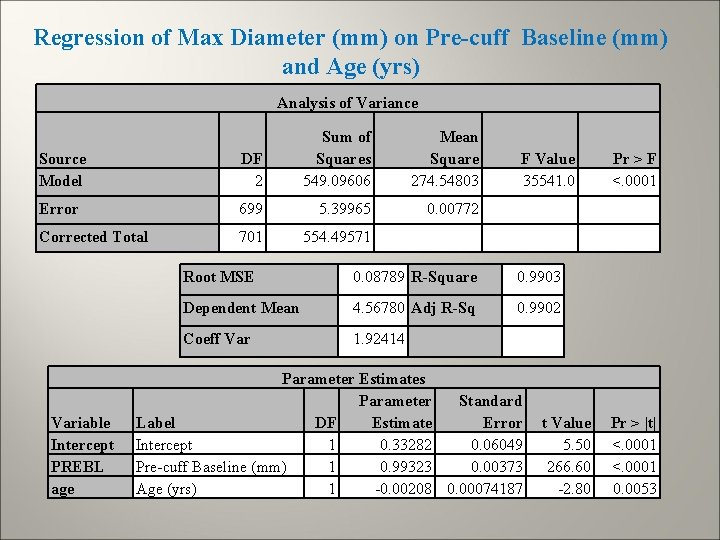
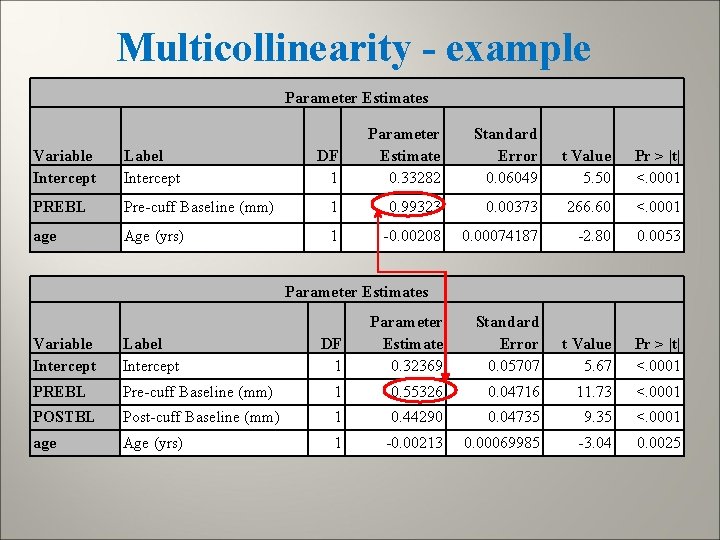
Regression of Max Diameter (mm) on Pre-cuff Baseline (mm) and Age (yrs) Analysis of Variance Source Model DF 2 Sum of Squares 549. 09606 Error 699 5. 39965 Corrected Total 701 554. 49571 Variable Intercept PREBL age Mean Square 274. 54803 0. 00772 F Value 35541. 0 Root MSE 0. 08789 R-Square 0. 9903 Dependent Mean 4. 56780 Adj R-Sq 0. 9902 Coeff Var 1. 92414 Parameter Estimates Parameter Standard Label DF Estimate Error Intercept 1 0. 33282 0. 06049 Pre-cuff Baseline (mm) 1 0. 99323 0. 00373 Age (yrs) 1 -0. 00208 0. 00074187 t Value 5. 50 266. 60 -2. 80 Pr > F <. 0001 Pr > |t| <. 0001 0. 0053

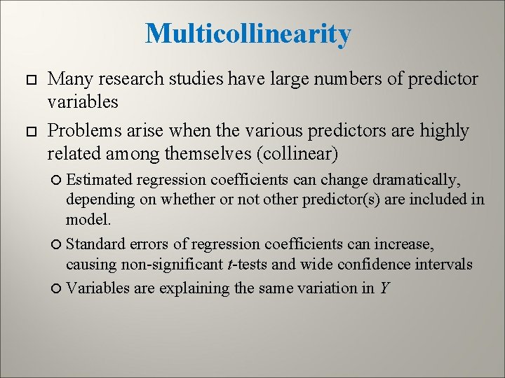
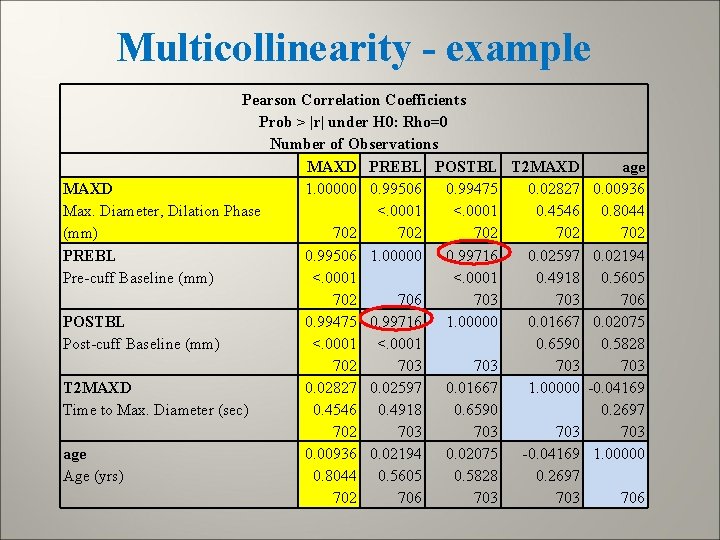
Multicollinearity Many research studies have large numbers of predictor variables Problems arise when the various predictors are highly related among themselves (collinear) Estimated regression coefficients can change dramatically, depending on whether or not other predictor(s) are included in model. Standard errors of regression coefficients can increase, causing non-significant t-tests and wide confidence intervals Variables are explaining the same variation in Y

Multicollinearity - example Pearson Correlation Coefficients Prob > |r| under H 0: Rho=0 Number of Observations MAXD PREBL POSTBL T 2 MAXD age MAXD 1. 00000 0. 99506 0. 99475 0. 02827 0. 00936 Max. Diameter, Dilation Phase <. 0001 0. 4546 0. 8044 (mm) 702 702 702 PREBL 0. 99506 1. 00000 0. 99716 0. 02597 0. 02194 Pre-cuff Baseline (mm) <. 0001 0. 4918 0. 5605 702 706 703 706 POSTBL 0. 99475 0. 99716 1. 00000 0. 01667 0. 02075 Post-cuff Baseline (mm) <. 0001 0. 6590 0. 5828 702 703 703 T 2 MAXD 0. 02827 0. 02597 0. 01667 1. 00000 -0. 04169 Time to Max. Diameter (sec) 0. 4546 0. 4918 0. 6590 0. 2697 702 703 703 age 0. 00936 0. 02194 0. 02075 -0. 04169 1. 00000 Age (yrs) 0. 8044 0. 5605 0. 5828 0. 2697 702 706 703 706

Multicollinearity - example Parameter Estimates DF 1 Parameter Estimate 0. 33282 Standard Error 0. 06049 t Value 5. 50 Pr > |t| <. 0001 Variable Intercept Label Intercept PREBL Pre-cuff Baseline (mm) 1 0. 99323 0. 00373 266. 60 <. 0001 age Age (yrs) 1 -0. 00208 0. 00074187 -2. 80 0. 0053 DF 1 Parameter Estimate 0. 32369 Standard Error 0. 05707 t Value 5. 67 Pr > |t| <. 0001 Parameter Estimates Variable Intercept Label Intercept PREBL Pre-cuff Baseline (mm) 1 0. 55326 0. 04716 11. 73 <. 0001 POSTBL Post-cuff Baseline (mm) 1 0. 44290 0. 04735 9. 35 <. 0001 age Age (yrs) 1 -0. 00213 0. 00069985 -3. 04 0. 0025

More About Assumptions We assume that the outcome (Y’s) are normally distributed. What assumptions have we made about the distribution of the IVs (the X’s)? None, except that they are RVs with some underlying distribution Recall, model assumption centers around the conditional distribution of Y’s (conditional on values of X’s) ANOVA is simply linear regression with series of dichotomous indicators for the “levels” of X

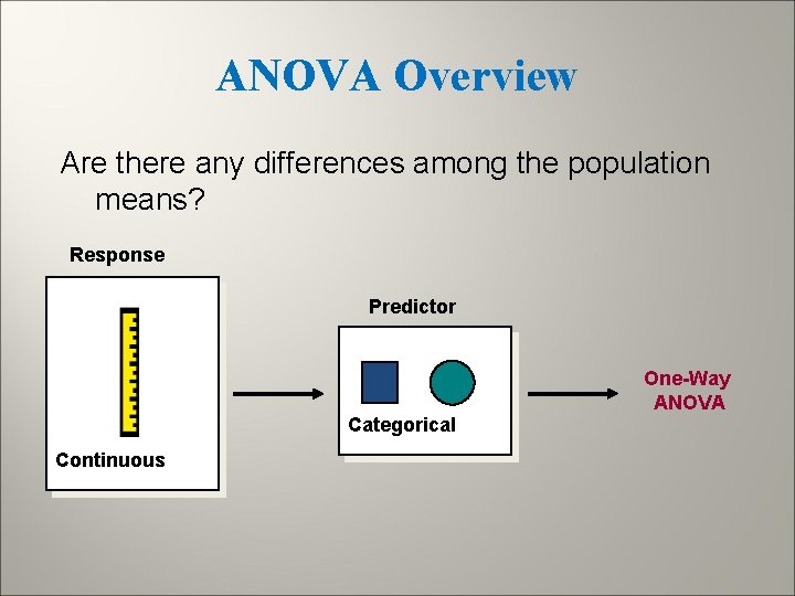
ANOVA Overview Are there any differences among the population means? Response Predictor One-Way ANOVA Categorical Continuous

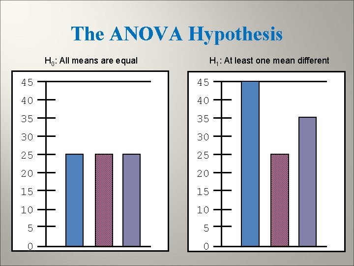
The ANOVA Hypothesis H 0: All means are equal H 1: At least one mean different 45 45 40 40 35 35 30 30 25 25 20 20 15 15 10 10 5 5 0 0

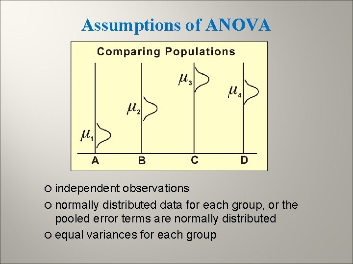
Assumptions of ANOVA independent observations normally distributed data for each group, or the pooled error terms are normally distributed equal variances for each group

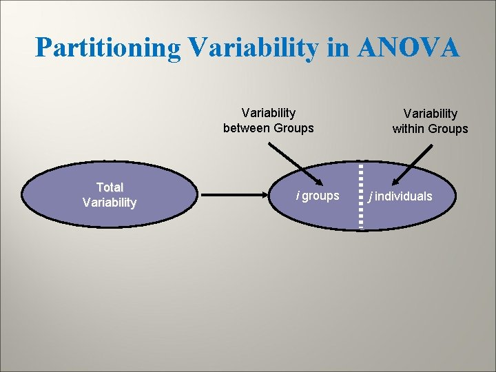
Partitioning Variability in ANOVA Variability between Groups Total Variability i groups Variability within Groups j individuals

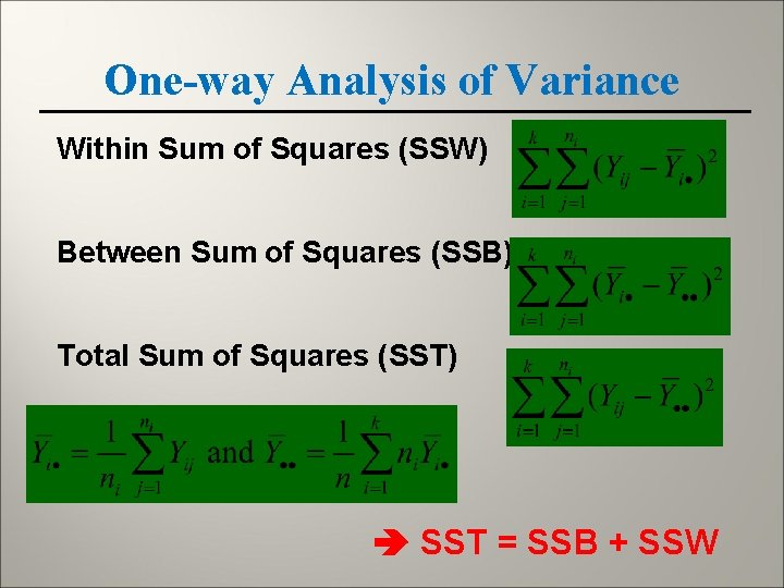
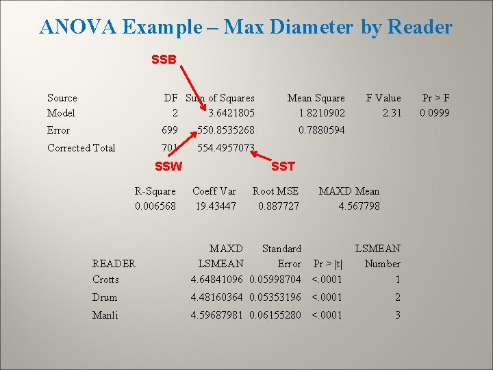
One-way Analysis of Variance Within Sum of Squares (SSW) Between Sum of Squares (SSB) Total Sum of Squares (SST) SST = SSB + SSW

ANOVA Example – Max Diameter by Reader SSB Source Model DF Sum of Squares 2 3. 6421805 Error 699 550. 8535268 Corrected Total 701 554. 4957073 SSW R-Square 0. 006568 Mean Square 1. 8210902 F Value 2. 31 0. 7880594 SST Coeff Var 19. 43447 Root MSE 0. 887727 MAXD Mean 4. 567798 READER Crotts MAXD Standard LSMEAN Error Pr > |t| 4. 64841096 0. 05998704 <. 0001 LSMEAN Number 1 Drum 4. 48160364 0. 05353196 <. 0001 2 Manli 4. 59687981 0. 06155280 <. 0001 3 Pr > F 0. 0999

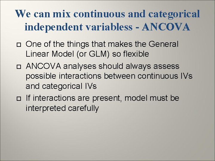
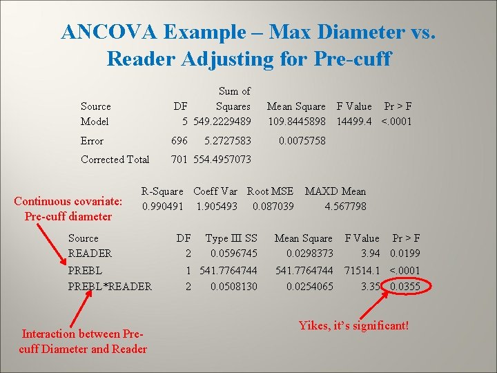
We can mix continuous and categorical independent variabless - ANCOVA One of the things that makes the General Linear Model (or GLM) so flexible ANCOVA analyses should always assess possible interactions between continuous IVs and categorical IVs If interactions are present, model must be interpreted carefully

ANCOVA Example – Max Diameter vs. Reader Adjusting for Pre-cuff Source Model Sum of DF Squares 5 549. 2229489 Error 696 Corrected Total 701 554. 4957073 Continuous covariate: Pre-cuff diameter 5. 2727583 Mean Square F Value Pr > F 109. 8445898 14499. 4 <. 0001 0. 0075758 R-Square Coeff Var Root MSE MAXD Mean 0. 990491 1. 905493 0. 087039 4. 567798 Source READER PREBL*READER Interaction between Precuff Diameter and Reader DF 2 Type III SS 0. 0596745 Mean Square 0. 0298373 F Value Pr > F 3. 94 0. 0199 1 541. 7764744 2 0. 0508130 541. 7764744 0. 0254065 71514. 1 <. 0001 3. 35 0. 0355 Yikes, it’s significant!

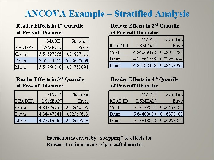
ANCOVA Example – Stratified Analysis Reader Effects in 1 st Quartile of Pre-cuff Diameter READER Crotts Drum Manli MAXD Standard LSMEAN Error 3. 50587755 0. 04807411 3. 51649412 0. 03650059 3. 50760000 0. 04759094 Reader Effects in 3 rd Quartile of Pre-cuff Diameter READER Crotts Drum Manli MAXD Standard LSMEAN Error 4. 84836735 0. 02640555 4. 84447541 0. 02366619 4. 77966667 0. 02667919 Reader Effects in 2 nd Quartile of Pre-cuff Diameter READER Crotts Drum Manli MAXD Standard LSMEAN Error 4. 24069492 0. 02395722 4. 25861538 0. 02282474 4. 28982456 0. 02437390 Reader Effects in 4 th Quartile of Pre-cuff Diameter READER Crotts Drum Manli MAXD Standard LSMEAN Error 5. 78133871 0. 06433425 5. 64400000 0. 06332105 5. 78918868 0. 06958252 Interaction is driven by “swapping” of effects for Reader at various levels of pre-cuff diameter.