LECTURE 4 Level set method and image segmentation

LECTURE 4 Level set method and image segmentation

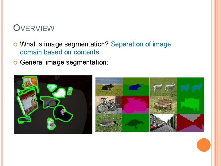
OVERVIEW What is image segmentation? Separation of image domain based on contents. General image segmentation:

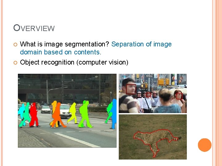
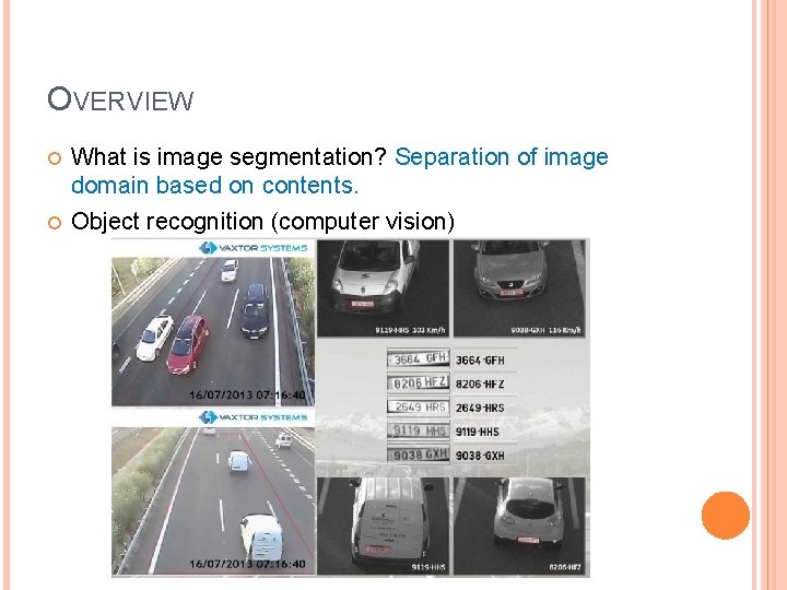
OVERVIEW What is image segmentation? Separation of image domain based on contents. Object recognition (computer vision)

OVERVIEW What is image segmentation? Separation of image domain based on contents. Object recognition (computer vision)

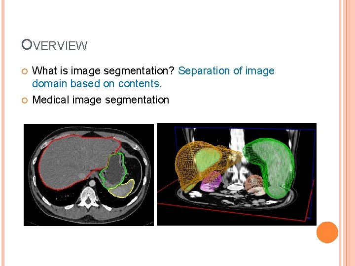
OVERVIEW What is image segmentation? Separation of image domain based on contents. Medical image segmentation

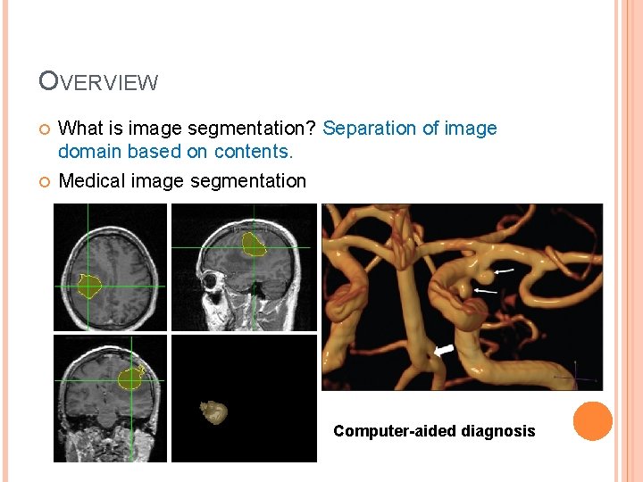
OVERVIEW What is image segmentation? Separation of image domain based on contents. Medical image segmentation Computer-aided diagnosis

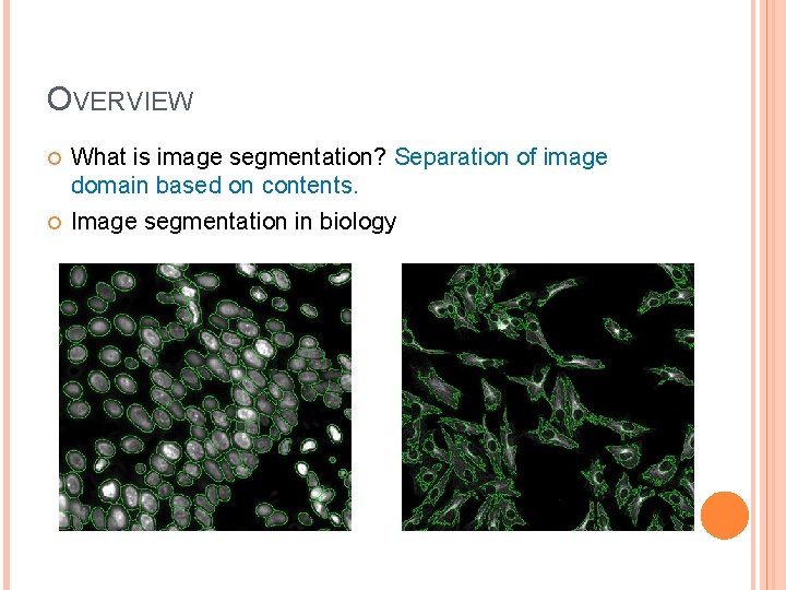
OVERVIEW What is image segmentation? Separation of image domain based on contents. Image segmentation in biology

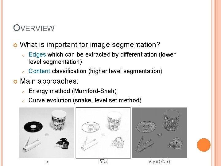
OVERVIEW What is important for image segmentation? o o Edges which can be extracted by differentiation (lower level segmentation) Content classification (higher level segmentation) Main approaches: o o Energy method (Mumford-Shah) Curve evolution (snake, level set method)

ENERGY METHOD Mumford-Shah (MS) Model

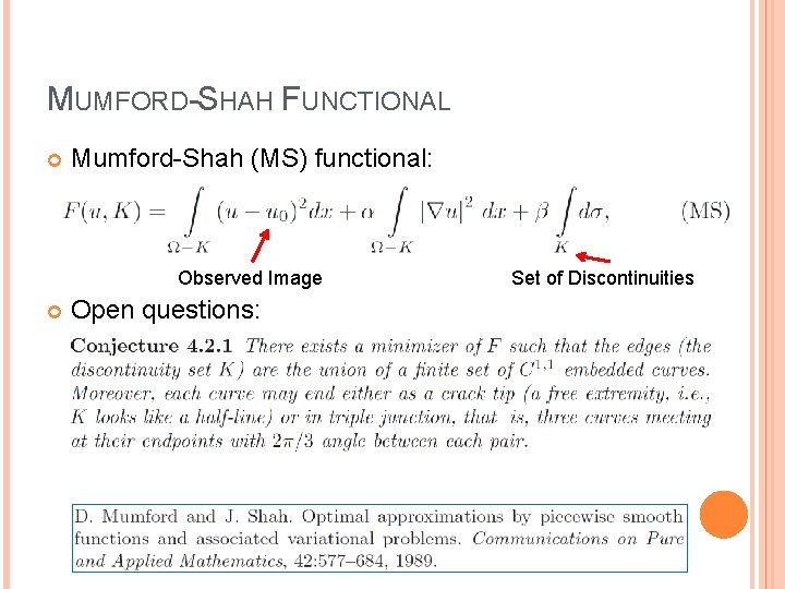
MUMFORD-SHAH FUNCTIONAL Mumford-Shah (MS) functional: Observed Image Open questions: Set of Discontinuities

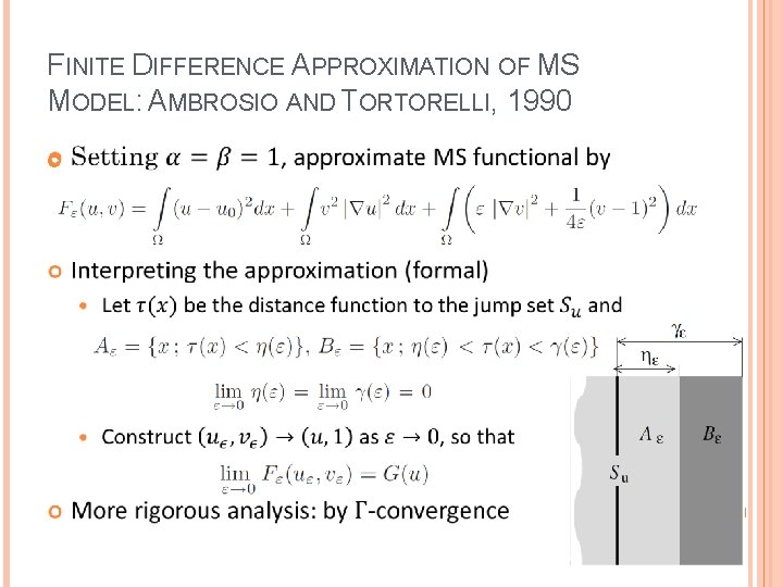
FINITE DIFFERENCE APPROXIMATION OF MS MODEL: AMBROSIO AND TORTORELLI, 1990

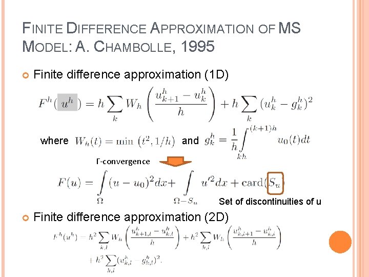
FINITE DIFFERENCE APPROXIMATION OF MS MODEL: A. CHAMBOLLE, 1995 Finite difference approximation (1 D) where and Γ-convergence Set of discontinuities of u Finite difference approximation (2 D)

CURVE EVOLUTION Snake, Geodesic Active-Contour, Chan-Vese Model, Level Set Method

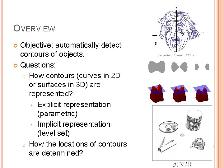
OVERVIEW Objective: automatically detect contours of objects. Questions: o How contours (curves in 2 D or surfaces in 3 D) are represented? • Explicit representation (parametric) • Implicit representation (level set) o How the locations of contours are determined?

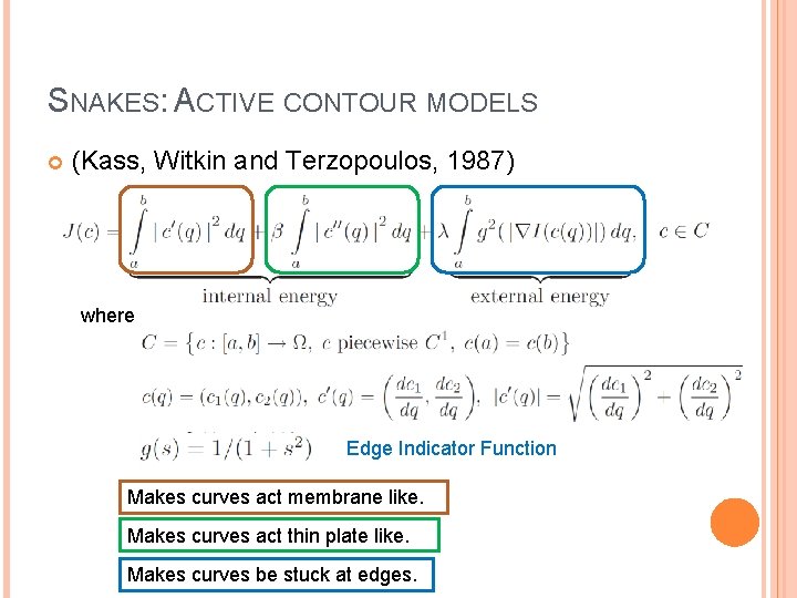
SNAKES: ACTIVE CONTOUR MODELS (Kass, Witkin and Terzopoulos, 1987) where Edge Indicator Function Makes curves act membrane like. Makes curves act thin plate like. Makes curves be stuck at edges.

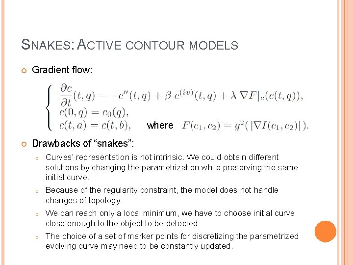
SNAKES: ACTIVE CONTOUR MODELS Gradient flow: where Drawbacks of “snakes”: o Curves’ representation is not intrinsic. We could obtain different solutions by changing the parametrization while preserving the same initial curve. o Because of the regularity constraint, the model does not handle changes of topology. o We can reach only a local minimum, we have to choose initial curve close enough to the object to be detected. o The choice of a set of marker points for discretizing the parametrized evolving curve may need to be constantly updated.

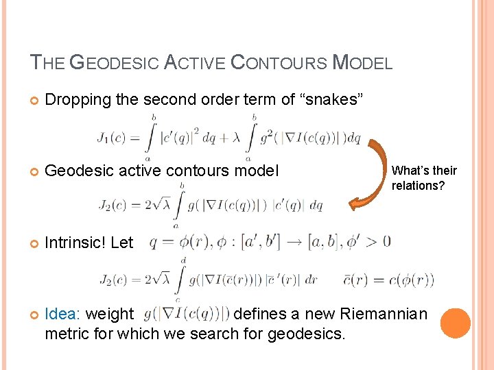
THE GEODESIC ACTIVE CONTOURS MODEL Dropping the second order term of “snakes” Geodesic active contours model Intrinsic! Let Idea: weight defines a new Riemannian metric for which we search for geodesics. What’s their relations?

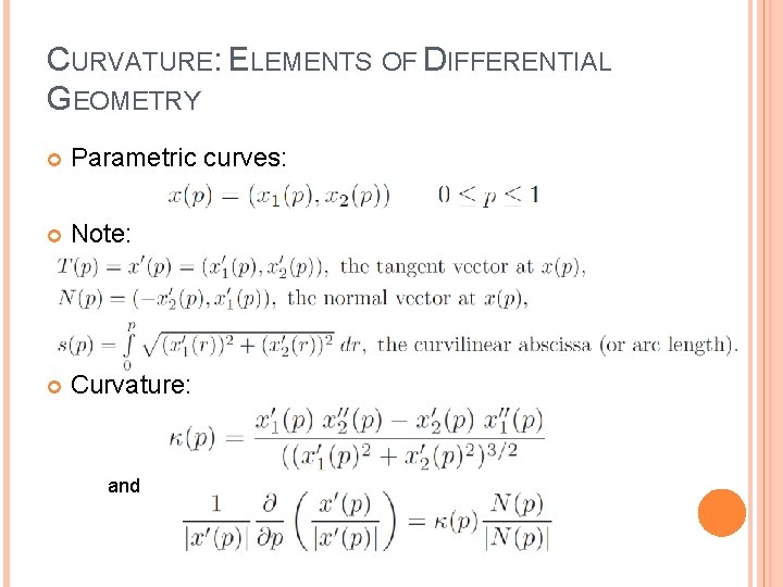
CURVATURE: ELEMENTS OF DIFFERENTIAL GEOMETRY Parametric curves: Note: Curvature: and

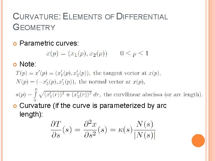
CURVATURE: ELEMENTS OF DIFFERENTIAL GEOMETRY Parametric curves: Note: Curvature (if the curve is parameterized by arc length):

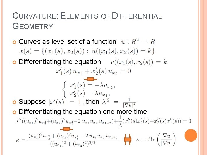
CURVATURE: ELEMENTS OF DIFFERENTIAL GEOMETRY Curves as level set of a function : Differentiating the equation Suppose , then Differentiating the equation one more time

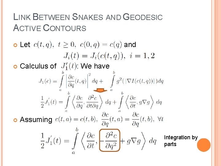
LINK BETWEEN SNAKES AND GEODESIC ACTIVE CONTOURS Let and Calculus of : We have Assuming : Integration by parts

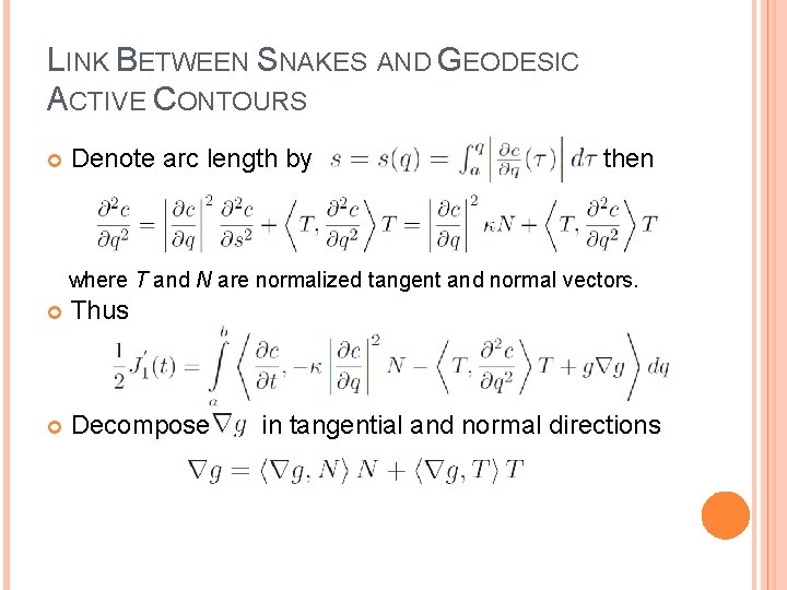
LINK BETWEEN SNAKES AND GEODESIC ACTIVE CONTOURS Denote arc length by , then where T and N are normalized tangent and normal vectors. Thus Decompose in tangential and normal directions

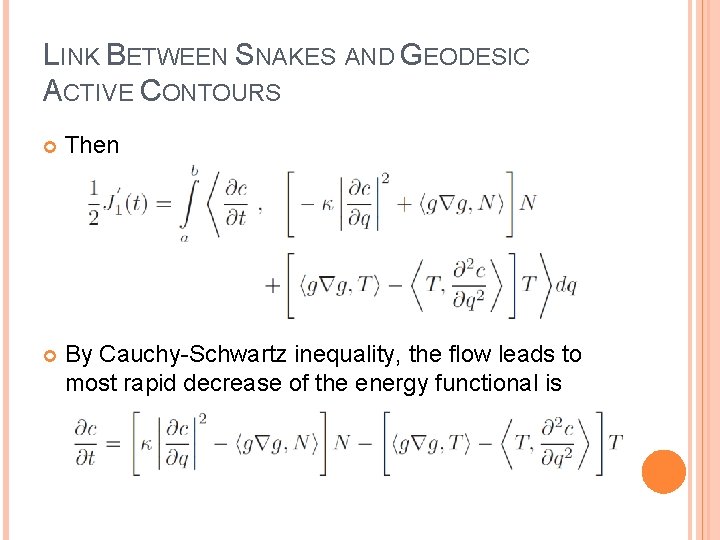
LINK BETWEEN SNAKES AND GEODESIC ACTIVE CONTOURS Then By Cauchy-Schwartz inequality, the flow leads to most rapid decrease of the energy functional is

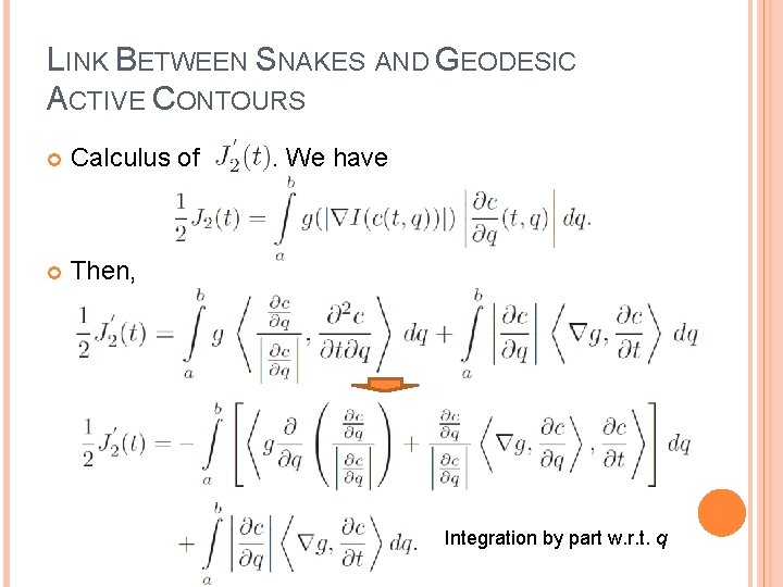
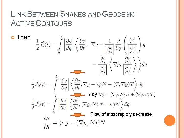
LINK BETWEEN SNAKES AND GEODESIC ACTIVE CONTOURS Calculus of . We have Then, Integration by part w. r. t. q

LINK BETWEEN SNAKES AND GEODESIC ACTIVE CONTOURS Then ( by ) Flow of most rapidly decrease

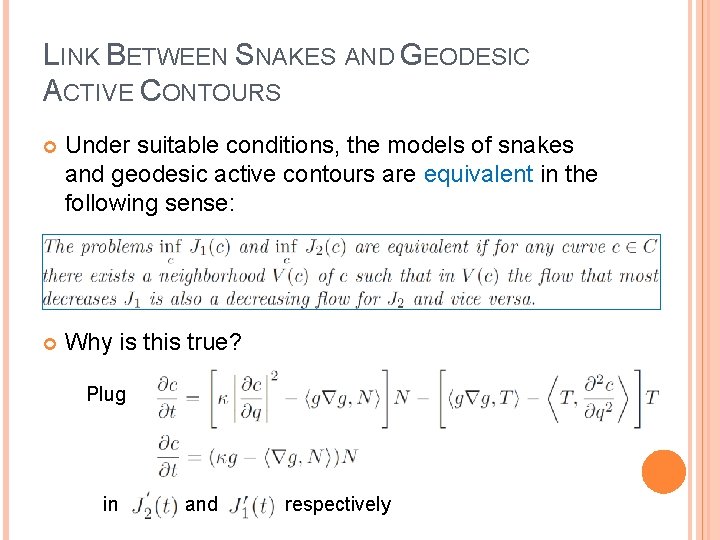
LINK BETWEEN SNAKES AND GEODESIC ACTIVE CONTOURS Under suitable conditions, the models of snakes and geodesic active contours are equivalent in the following sense: Why is this true? Plug in and respectively

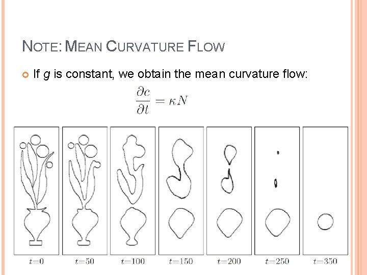
NOTE: MEAN CURVATURE FLOW If g is constant, we obtain the mean curvature flow:

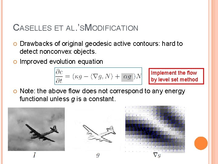
CASELLES ET AL. ’S MODIFICATION Drawbacks of original geodesic active contours: hard to detect nonconvex objects. Improved evolution equation Implement the flow by level set method Note: the above flow does not correspond to any energy functional unless g is a constant.

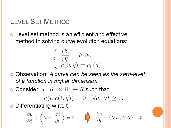
LEVEL SET METHOD Level set method is an efficient and effective method in solving curve evolution equations: Observation: A curve can be seen as the zero-level of a function in higher dimension. Consider such that Differentiating w. r. t. t

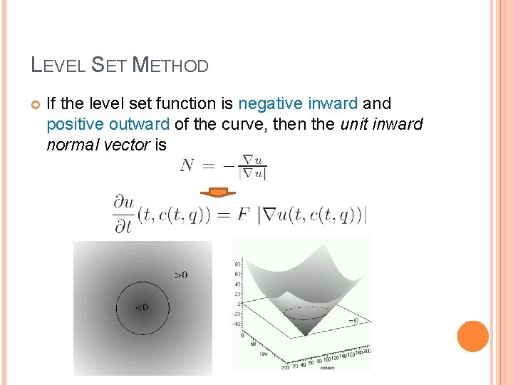
LEVEL SET METHOD If the level set function is negative inward and positive outward of the curve, then the unit inward normal vector is

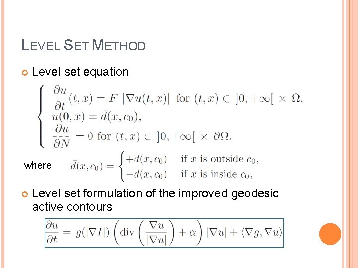
LEVEL SET METHOD Level set equation where Level set formulation of the improved geodesic active contours

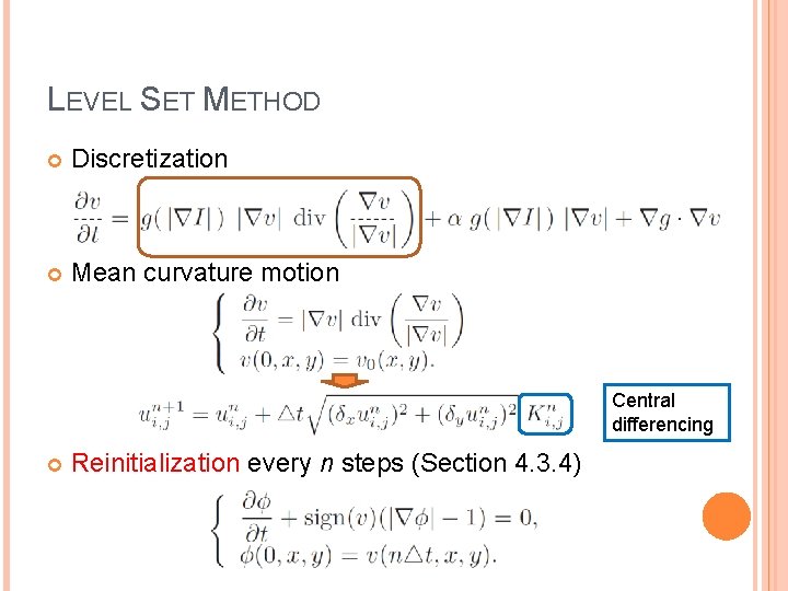
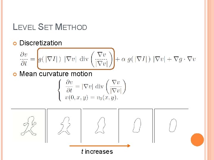
LEVEL SET METHOD Discretization Mean curvature motion Central differencing Reinitialization every n steps (Section 4. 3. 4)

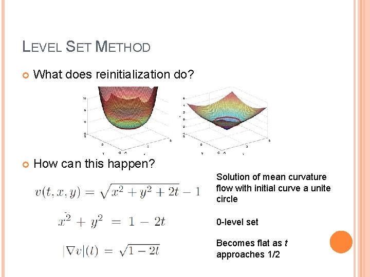
LEVEL SET METHOD What does reinitialization do? How can this happen? Solution of mean curvature flow with initial curve a unite circle 0 -level set Becomes flat as t approaches 1/2

LEVEL SET METHOD Discretization Mean curvature motion t increases

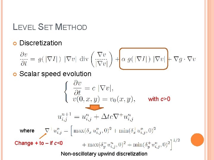
LEVEL SET METHOD Discretization Scalar speed evolution with c>0 where Change + to – if c<0 Non-oscillotary upwind discretization

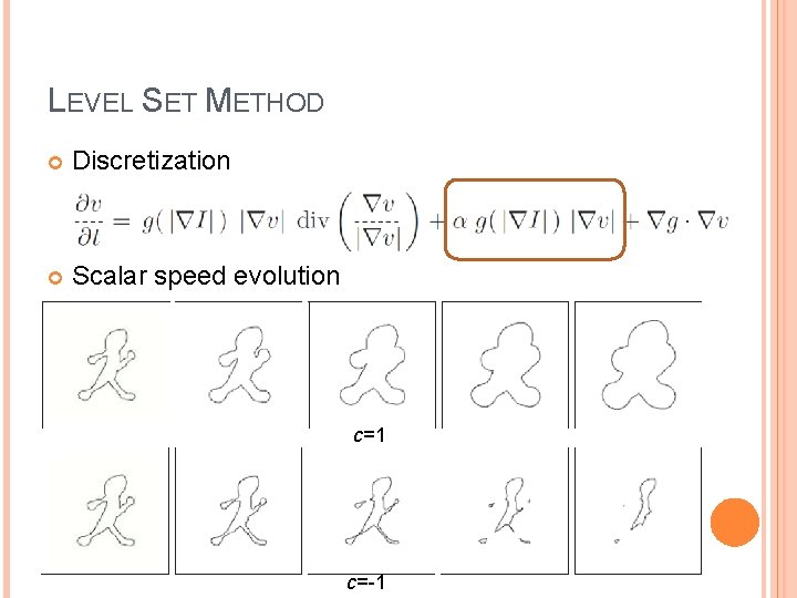
LEVEL SET METHOD Discretization Scalar speed evolution c=1 c=-1

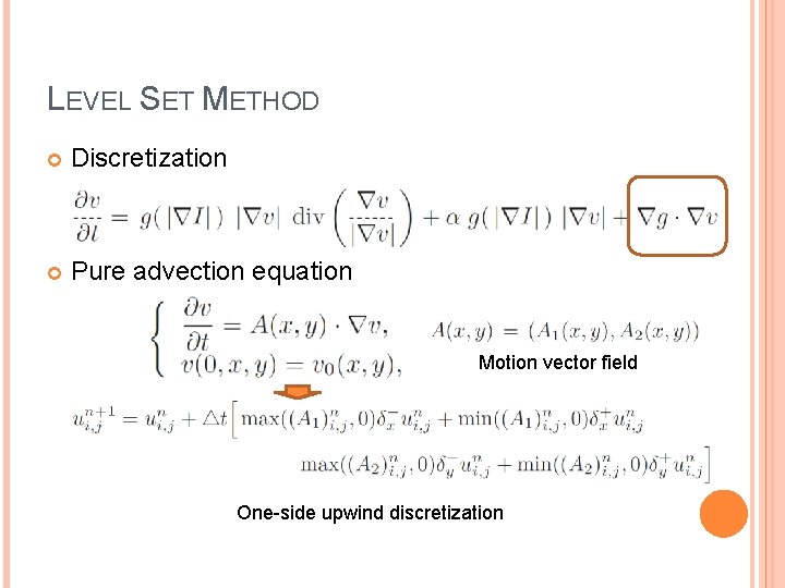
LEVEL SET METHOD Discretization Pure advection equation Motion vector field One-side upwind discretization

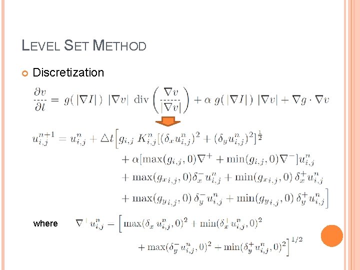
LEVEL SET METHOD Discretization where

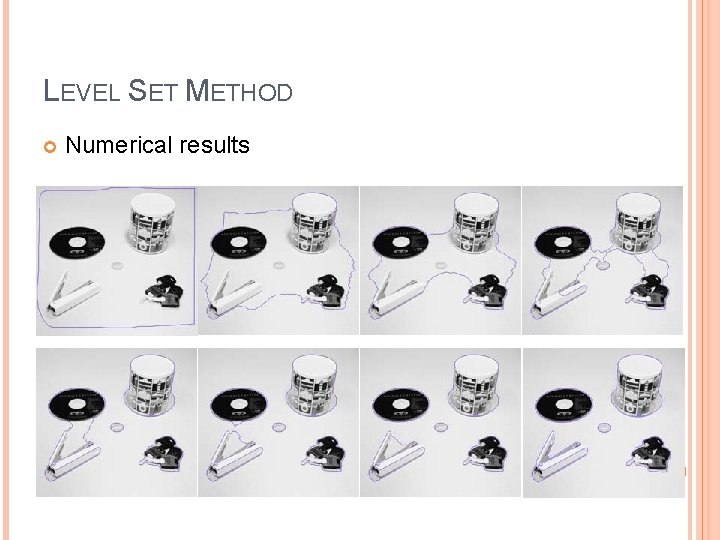
LEVEL SET METHOD Numerical results

BRAIN ANEURYSM SEGMENTATION B. Dong et al. , Level set based brain aneurysm capturing in 3 D, Inverse Problems and Imaging, 4(2), 241 -255, 2010.

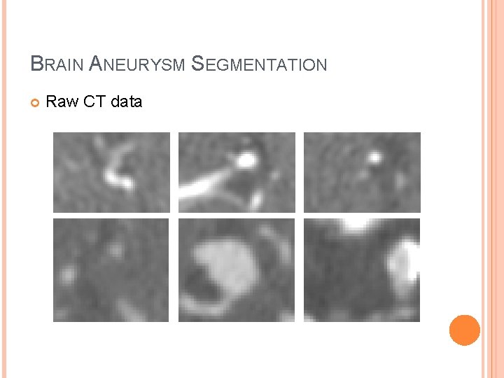
BRAIN ANEURYSM SEGMENTATION Raw CT data

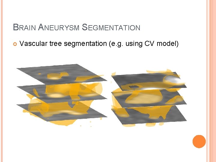
BRAIN ANEURYSM SEGMENTATION Vascular tree segmentation (e. g. using CV model)

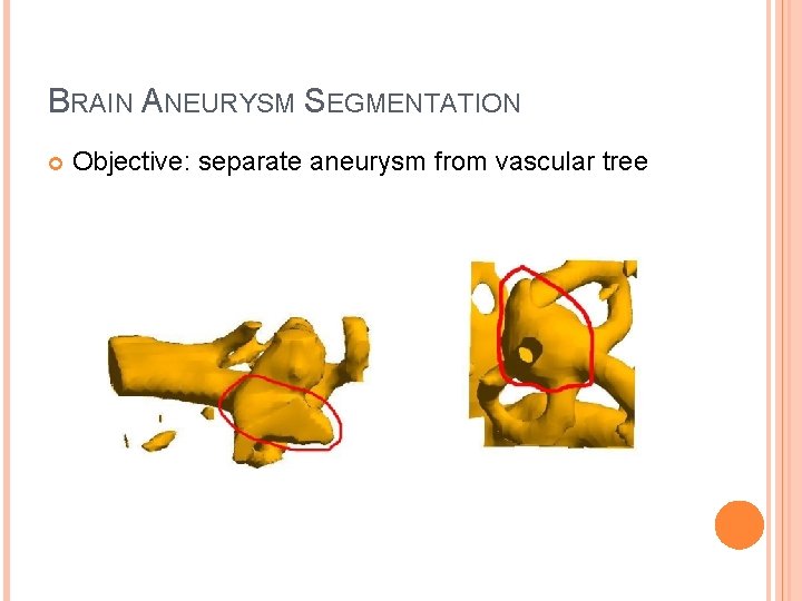
BRAIN ANEURYSM SEGMENTATION Objective: separate aneurysm from vascular tree

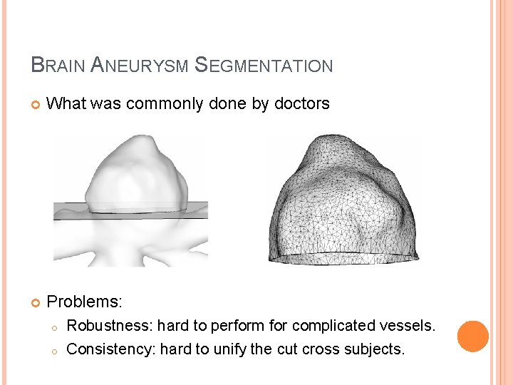
BRAIN ANEURYSM SEGMENTATION What was commonly done by doctors Problems: o o Robustness: hard to perform for complicated vessels. Consistency: hard to unify the cut cross subjects.

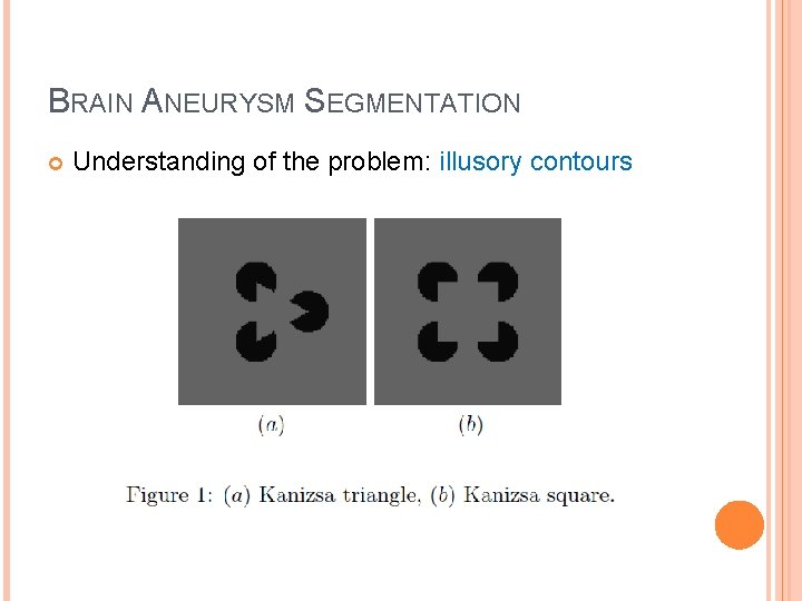
BRAIN ANEURYSM SEGMENTATION Understanding of the problem: illusory contours

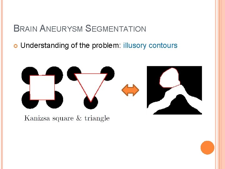
BRAIN ANEURYSM SEGMENTATION Understanding of the problem: illusory contours

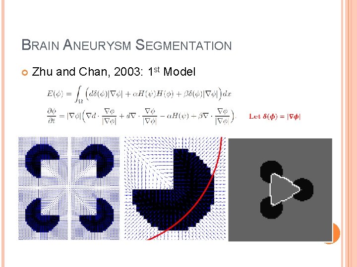
BRAIN ANEURYSM SEGMENTATION Zhu and Chan, 2003: 1 st Model

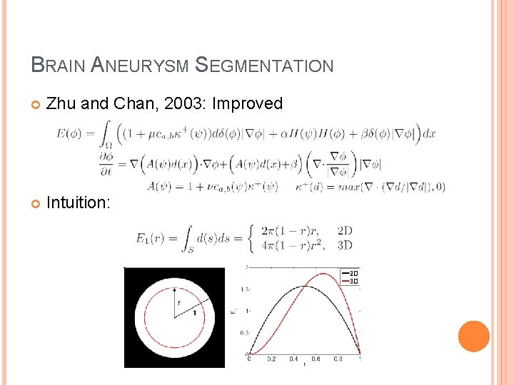
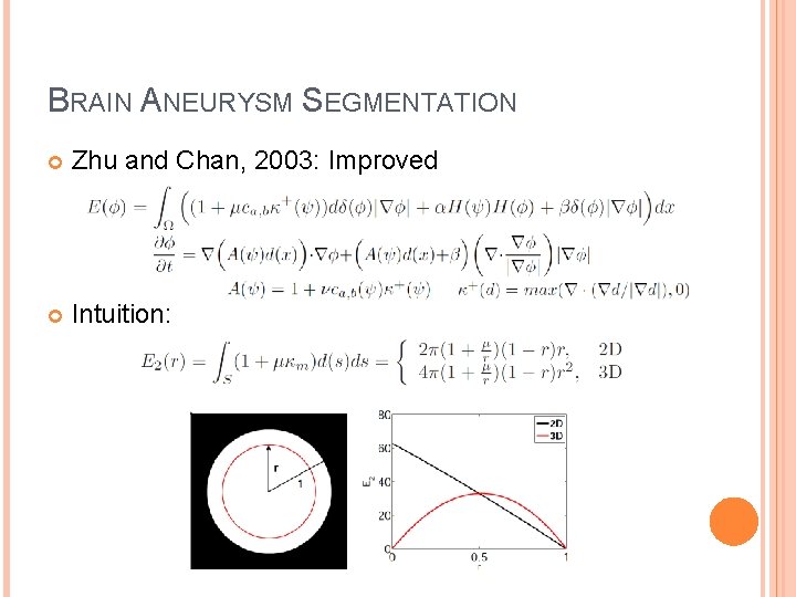
BRAIN ANEURYSM SEGMENTATION Zhu and Chan, 2003: Improved Intuition:

BRAIN ANEURYSM SEGMENTATION Zhu and Chan, 2003: Improved Intuition:

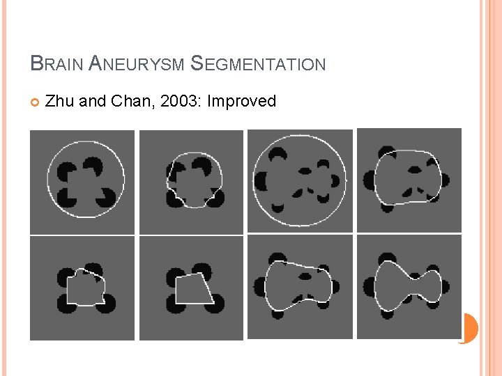
BRAIN ANEURYSM SEGMENTATION Zhu and Chan, 2003: Improved

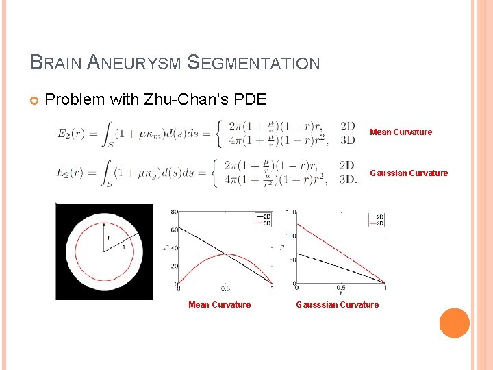
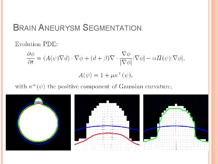
BRAIN ANEURYSM SEGMENTATION Problem with Zhu-Chan’s PDE Mean Curvature Gaussian Curvature Mean Curvature Gausssian Curvature

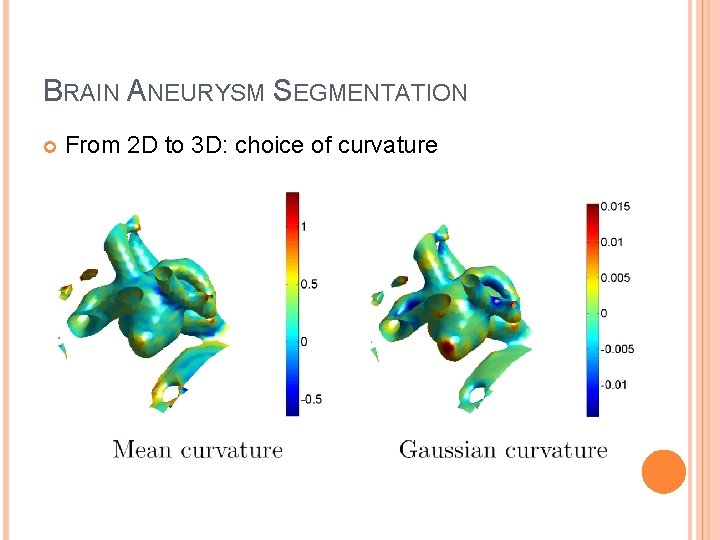
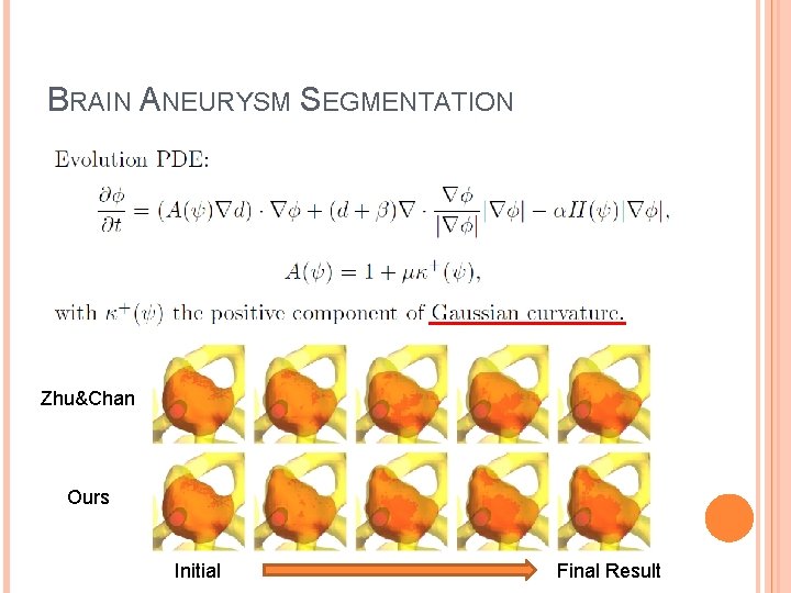
BRAIN ANEURYSM SEGMENTATION From 2 D to 3 D: choice of curvature

BRAIN ANEURYSM SEGMENTATION

BRAIN ANEURYSM SEGMENTATION Zhu&Chan Ours Initial Final Result

ENERGY METHOD - REVISITED Approximations of Mumford-Shah Model

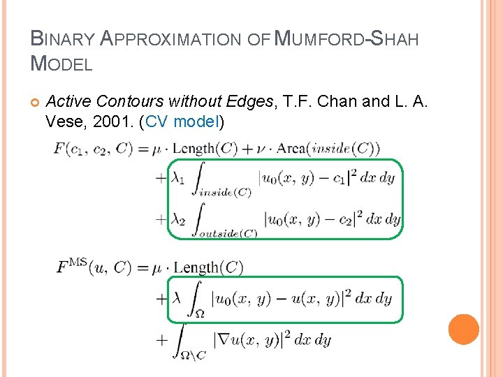
BINARY APPROXIMATION OF MUMFORD-SHAH MODEL Active Contours without Edges, T. F. Chan and L. A. Vese, 2001. (CV model)

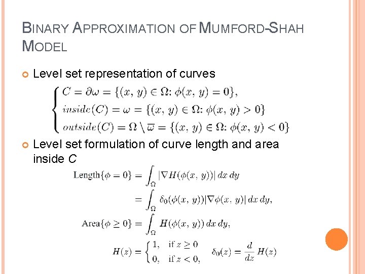
BINARY APPROXIMATION OF MUMFORD-SHAH MODEL Level set representation of curves Level set formulation of curve length and area inside C

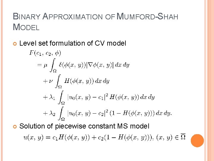
BINARY APPROXIMATION OF MUMFORD-SHAH MODEL Level set formulation of CV model Solution of piecewise constant MS model

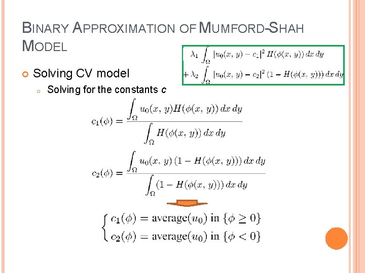
BINARY APPROXIMATION OF MUMFORD-SHAH MODEL Solving CV model o Solving for the constants c

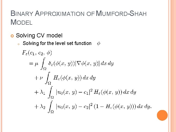
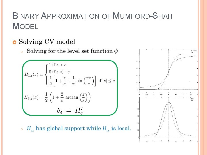
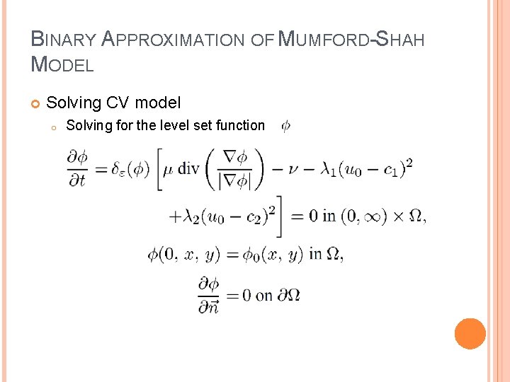
BINARY APPROXIMATION OF MUMFORD-SHAH MODEL Solving CV model o Solving for the level set function

BINARY APPROXIMATION OF MUMFORD-SHAH MODEL

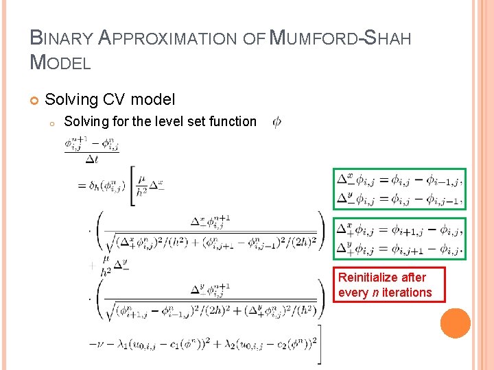
BINARY APPROXIMATION OF MUMFORD-SHAH MODEL Solving CV model o Solving for the level set function

BINARY APPROXIMATION OF MUMFORD-SHAH MODEL Solving CV model o Solving for the level set function Reinitialize after every n iterations

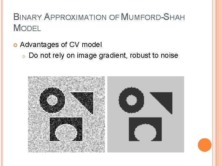
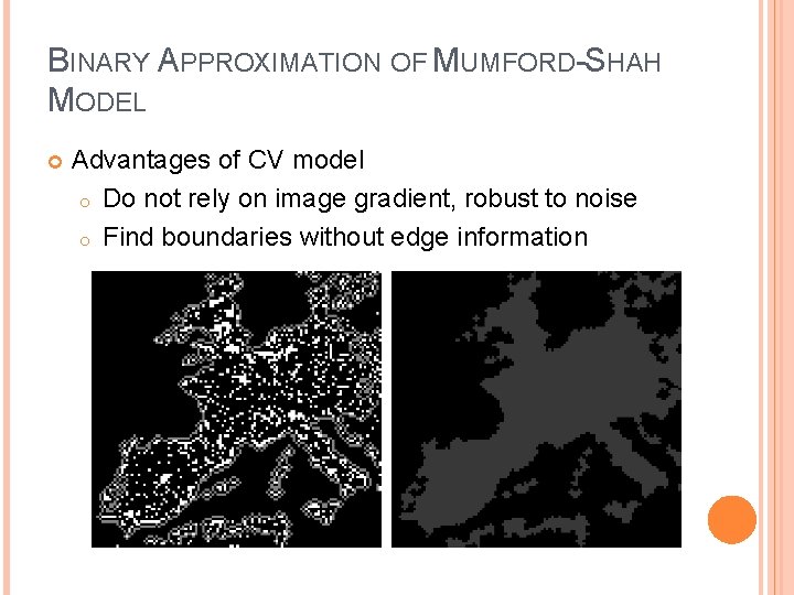
BINARY APPROXIMATION OF MUMFORD-SHAH MODEL Advantages of CV model o Do not rely on image gradient, robust to noise

BINARY APPROXIMATION OF MUMFORD-SHAH MODEL Advantages of CV model o Do not rely on image gradient, robust to noise o Find boundaries without edge information

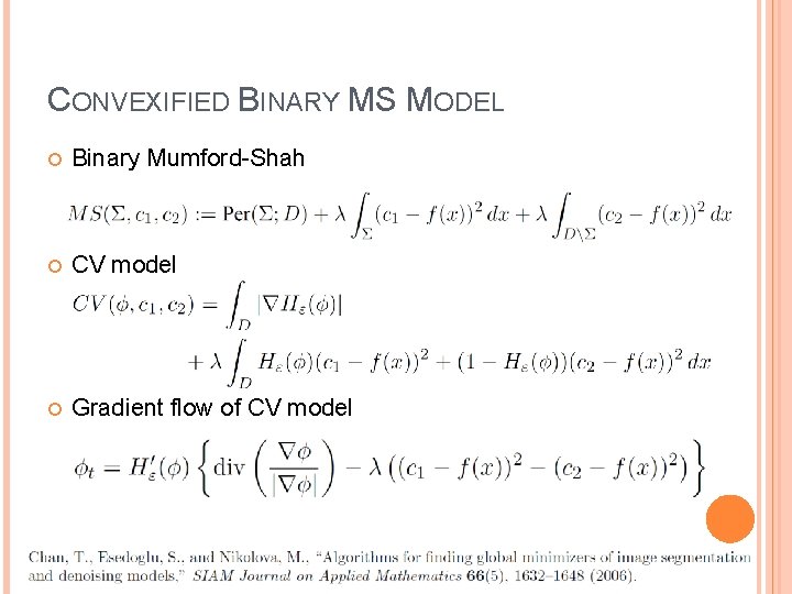
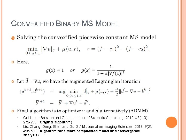
CONVEXIFIED BINARY MS MODEL Binary Mumford-Shah CV model Gradient flow of CV model

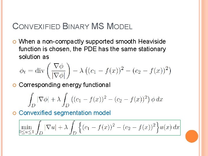
CONVEXIFIED BINARY MS MODEL When a non-compactly supported smooth Heaviside function is chosen, the PDE has the same stationary solution as Corresponding energy functional Convexified segmentation model

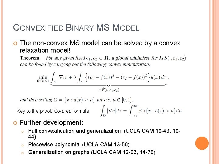
CONVEXIFIED BINARY MS MODEL The non-convex MS model can be solved by a convex relaxation model! Key to the proof: Co-area formula Further development: o o o Full convexification and generalization (UCLA CAM 10 -43, 1044) Piecewise polynomial (UCLA CAM 13 -50) Generalization on graphs (UCLA CAM 12 -03, 14 -79)

CONVEXIFIED BINARY MS MODEL • • Goldstein, Bresson and Osher. Journal of Scientific Computing, 2010, 45(1 -3): 272 -293. (Original algorithm) Liu, Zhang, Dong, Shen and Gu. SIAM Journal on Imaging Sciences, 2016, 9(2): 495 -536. (Algorithm for a more complicated model and convergence analysis)

HOMEWORK 3 Implement the geodesic active contours model using level set formulation (ppt page 35 -38). Implement the original CV model (ppt page 60 -64) Implement the convexified CV model (ppt page 70). Use images of your own selection Observe: o Segmentation results for different types of images o Effects of noise and blur on the results o Comparison between the three models Note: codes of reinitialization is provided.