Lecture 4 Basics Of Macroeconomics I Dr Rajeev

Lecture 4: Basics Of Macroeconomics I Dr. Rajeev Dhawan Director Given to the EMBA 8400 Class Buckhead Center April 3, 2010

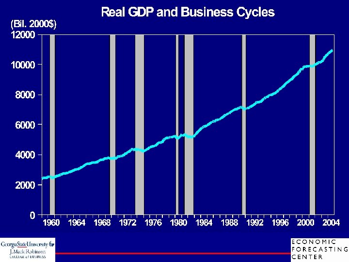
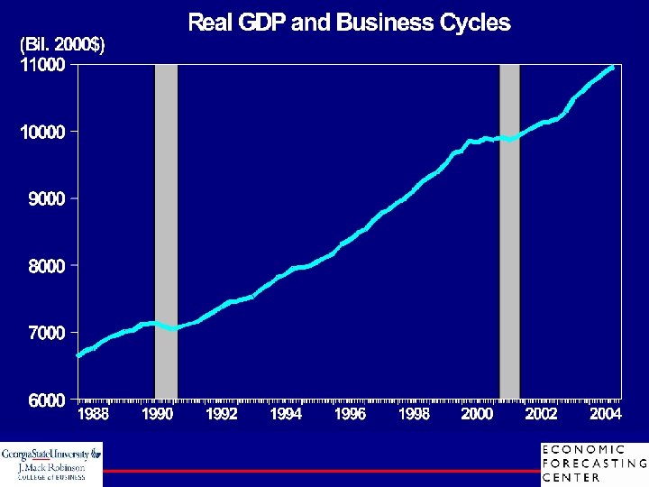
Article: Business Cycles BUSINESS CYCLE REFERENCE DATES Peak DURATION IN MONTHS Trough Quarterly dates are in parentheses Contraction Expansion Cycle Peak to Trough Previous trough to this peak Trough from Previous Trough Peak from Previous Peak May 1937(II) February 1945(I) November 1948(IV) July 1953(II) August 1957(III) June 1938 (II) October 1945 (IV) October 1949 (IV) May 1954 (II) April 1958 (II) 13 8 11 10 8 50 80 37 45 39 63 88 48 55 47 93 93 45 56 49 April 1960(II) December 1969(IV) November 1973(IV) January 1980(I) July 1981(III) February 1961 (I) November 1970 (IV) March 1975 (I) July 1980 (III) November 1982 (IV) 10 11 16 6 16 24 106 36 58 12 34 117 52 64 28 32 116 47 74 18 July 1990(III) March 1991(I) 8 92 100 108 March 2001 (I) November 2001 (IV) 8 120 128 NBER Report Cycle Dates 2003

Mar 01’ ~ Nov 01’ 9 -0. 1% Forecast of the Nation, 2003 -4. 0% 4. 2 5. 6

Article: NBER’s FAQs Q: The financial press often states the definition of a recession as two consecutive quarters of decline in real GDP. How does that relate to the NBER's recession dating procedure? – Most of the recessions identified by our procedures consist of two or more quarters of declining real GDP, but not all of them – We consider the depth as well as the duration of the decline in economic activity. – Second, we use a broader array of indicators than just real GDP – Third, we use monthly indicators to arrive at a monthly chronology Q: Could you give an example illustrating this point? – The two-quarter-decline rule of thumb would not have allowed the declaration of the recession until August 2002 Q: How does the NBER balance the differing behavior of employment and output? – There is no fixed rule for how the different indicators are weighted

Article: NBER’s FAQs Q. You emphasize the payroll survey as a source for data on economy-wide employment. What about the household survey? – Although the household survey is a large, well-designed probability sample of the U. S. population, its estimates of total employment appear to be noisier than those from the payroll survey Q. How do the movements of unemployment claims inform the Bureau's thinking? – A bulge in jobless claims would appear to forecast declining employment, but we do not use forecasts and the claims numbers have a lot of noise Q: What about the unemployment rate? – Unemployment is generally a lagging indicator. Its rise from a very low level to date is consistent with the employment data

Peak & Trough Announcements The November 2001 trough was announced July 17, 2003. The March 2001 peak was announced November 26, 2001. The March 1991 trough was announced December 22, 1992. The July 1990 peak was announced April 25, 1991. The November 1982 trough was announced July 8, 1983. The July 1981 peak was announced January 6, 1982. The July 1980 trough was announced July 8, 1981. The January 1980 peak was announced June 3, 1980.

2001 Recession vs. History For Details Refer: http: //www. nber. org/

Real GDP and Consumption FRBSF Economic Letter, June 2003

Investment and Stock Market FRBSF Economic Letter, June 2003

Chapter 24 Measuring the Cost of Living

Consumer Price Index & Inflation ¨ Inflation refers to a situation in which the economy’s overall price level is rising. ¨ The inflation rate is the percentage change in the price level from the previous period. ¨ The Consumer Price Index (CPI) is a measure of the overall cost of goods and services bought by a typical consumer (produced by BLS). ¨ Inflation rate is change in CPI.

Steps to Calculate CPI Index ¨ Fix the Basket: Determine what prices are most important to the typical consumer. – The Bureau of Labor Statistics (BLS) identifies a market basket of goods and services the typical consumer buys. – The BLS conducts monthly consumer surveys to set the weights for the prices of those goods and services. ¨ Find the Prices: Find the prices of each of the goods and services in the basket for each point in time. ¨ Compute the Basket's Cost: Use the data on prices to calculate the cost of the basket of goods and services at different times. ¨ Choose a Base Year and Compute the Index:

Steps to Calculate CPI Index ¨ Choose a Base Year and Compute the Index: – Designate one year as the base year, making it the benchmark against which other years are compared. – Compute the index by dividing the price of the basket in one year by the price in the base year and multiplying by 100.

How the Inflation Rate Is Calculated ¨ The Inflation Rate – The inflation rate is calculated as follows:

Calculating the Consumer Price Index and the Inflation Rate: An Example

Calculating the Consumer Price Index and the Inflation Rate: An Example

Another Example of CPI and Inflation Calculations ¨ Calculating the Consumer Price Index and the Inflation Rate: – Base Year is 2002. – Basket of goods in 2002 costs $1, 200. – The same basket in 2003 costs $1, 236. – CPI = ($1, 236/$1, 200) 100 = 103. – Prices increased 3 percent between 2002 and 2003.

FYI: What Is in the CPI’s Basket? 17% Transportation 15% Food and beverages Education and communication 6% 42% Housing 6% 6% 4% 4% Medical care Recreation Apparel Other goods and services

The GDP Deflator vs. CPI ¨ The BLS calculates other prices indexes: – The index for different regions within the country. – The producer price index, which measures the cost of a basket of goods and services bought by firms rather than consumers.

CPI and GDP Deflator Percent per Year 15 CPI 10 5 0 GDP deflator 1965 1970 1975 1980 1985 1990 1995 2000

Problems in Measuring CPI ¨ Substitution bias ¨ Introduction of new goods ¨ Unmeasured quality changes

Use of Price Indexes ¨ Price indexes are used to correct for the effects of inflation when comparing dollar figures from different times. ¨ Do the following to convert (inflate) Babe Ruth’s wages in 1931 to dollars in 2005:

The Most Popular Movies of All Times, Inflation Adjusted

Real and Nominal Interest Rates ¨ The nominal interest rate is the interest rate usually reported and not corrected for inflation. – This is the interest rate that a bank pays. ¨ The real interest rate is the nominal interest rate that is corrected for the effects of inflation.

Real and Nominal Interest Rates You borrow $1, 000 for one year. Nominal interest rate is 15%. During the year inflation is 10%. Real interest rate = Nominal interest rate – Inflation = 15% - 10% = 5%
 15% Nominal interest rate 10 5")
Real and Nominal Interest Rates (percent per year) 15% Nominal interest rate 10 5 0 Real interest rate -5 1965 1970 1975 1980 1985 1990 1995 2000 2005

Chapter 26 Saving, Investment and the Financial System

Tax Cuts have Eased the Oil Price Shock This Time Source: Prof. Larry J. Kimbell, Nov. 2004
 has been")
Savings And National Income Math ¨ GDP (as the sum of expenditures) has been defined as: Y = C + I + G + NX In a closed economy: Y=C+I+G ¨ Rearranging terms gives: Y-C-G=I ¨ The left-hand side, which is the nation's income (GDP) leftover after consumption and government spending, is defined as National Savings. Since Y - C - G is defined as being equal to "S": S=I

Continued. . ¨ This relationship must hold for the economy as a whole (when the economy is closed). Now, with S=Y-C-G ¨ Add and subtract the government's tax revenue (T) to the right-hand side S=Y-C-G+T-T ¨ Then rearrange terms on the right hand side to get S = (Y - T - C) + (T - G)

Continued. . ¨ This expression breaks down national savings into two components: private savings and public savings. ¨ Private savings (Y - T - C) is the income left in the economy after taxes and consumption have each been paid for. ¨ Public savings (T - G) is equal to the taxes collected by the government, minus government spending. This is also an expression for the government surplus/deficit (surplus if T > G, deficit if T < G).

Market For Loanable Funds Interest Rate Supply 5% Demand 0 $1, 200 Loanable Funds (in billions of dollars)

Increase in Supply of Loanable Funds Interest Rate Policy 1: Saving Incentives Supply, S 1 S 2 1. Tax incentives for saving increase the supply of loanable funds. . . 5% 4% 2. . which reduces the equilibrium interest rate. . . Demand 0 $1, 200 $1, 600 3. . and raises the equilibrium quantity of loanable funds. Loanable Funds (in billions of dollars)

Increase in Demand of Loanable Funds Interest Rate Policy 2: Investment Incentives Supply 1. An investment tax credit increases the demand for loanable funds. . . 6% 5% 2. . which raises the equilibrium interest rate. . . 0 D 2 Demand, D 1 $1, 200 $1, 400 3. . and raises the equilibrium quantity of loanable funds. Loanable Funds (in billions of dollars)

Effect Of A Government Budget Deficit Policy 3: Budget Deficit Interest Rate S 2 Supply, S 1 1. A budget deficit decreases the supply of loanable funds. . . 6% 5% 2. . which raises the equilibrium interest rate. . . Demand 0 $800 $1, 200 3. . and reduces the equilibrium quantity of loanable funds. Loanable Funds (in billions of dollars)

The U. S. Government Debt Percent of GDP 120 World War II 100 80 60 Revolutionary War 40 Civil War World War I 20 0 1790 1810 1830 1850 1870 1890 1910 1930 1950 1970 1990 2010 Copyright© 2004 South-Western
- Slides: 47