LECTURE 4 Assoc Prof Dr Yasemin Asu rpc

LECTURE 4 Assoc. Prof. Dr. Yasemin Asu Çırpıcı, YTU, Department of Economics

� Working on networks we are usually interested in not only analyze the real‐world networks but also modeling the networks. � Why is so? � Why to model networks? �A model is a simple representation of a complex real‐world network. � It will allow us to test certain assumptions. � We will be able to do this by implementing those assumptions to our model and see whether the model of ours really resembles the real network that we observe. https: //www. youtube. com/watch? v=3 Pxte. Ag. Vf 0 o

� Suppose we analyze a social network and observe that some people have much more friends than others. � You may say that what leads to this result is just random fluctuations. � People form random links and this leads to some people having much more friends. � Next, you can test this. � You can generate a network according to your model and see if indeed you get some individuals who have many more friends than others.

� If it doesn’t happen, if the model can not reproduce the distribution of degrees of the real network this means that your model needs to be adjusted. � The way you think is not what really happens. � The model needs to be extended. � If you find out that the real network has properties not close to a random network then you may say well this is worth analyzing and you will proceed.

� Random networks are very basic of the models that we will cover. � Paul Erdős and Alféd Rényi introduced these models (1959).

� Before Paul Erdős and Alfréd Rényi graph theory mostly focused on regular graphs. But for the studies concerning the complex systems regular graphs are the exception rather than the norm. What Erdős and Rényi did was to introduce randomness in this field.

� Think of a spread of a disease. It will depend on the average interconnections and also to the distribution of them. � So, it will depend on how many people are in connection and does everyone interact with about the same number of people, or do someone have connection with very large numbers while others have very few. � Random graphs can serve as a useful tool for modeling such cases (Jackson, 2008).

� In a random graph, every edge is formed with probability independently of every other edge. � So, two nodes are connected with a given probability p.

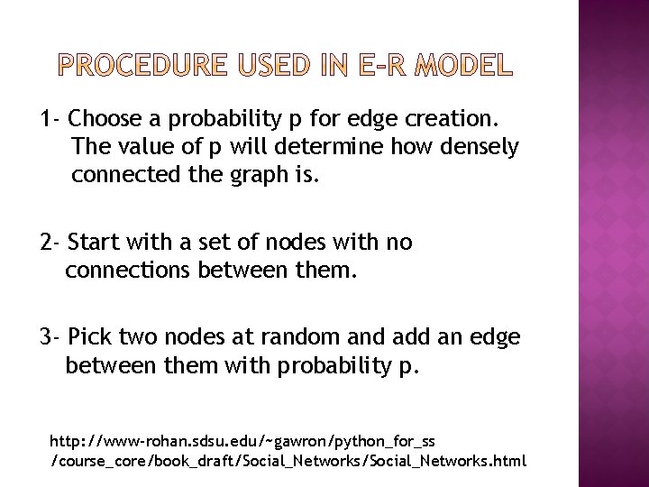
1‐ Choose a probability p for edge creation. The value of p will determine how densely connected the graph is. 2‐ Start with a set of nodes with no connections between them. 3‐ Pick two nodes at random and add an edge between them with probability p. http: //www‐rohan. sdsu. edu/~gawron/python_for_ss /course_core/book_draft/Social_Networks. html

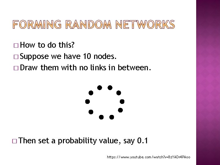
� How to do this? � Suppose we have 10 nodes. � Draw them with no links in between. � Then set a probability value, say 0. 1 https: //www. youtube. com/watch? v=8 z. YADr 4 PAoo

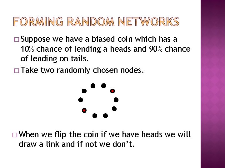
� Suppose we have a biased coin which has a 10% chance of lending a heads and 90% chance of lending on tails. � Take two randomly chosen nodes. � When we flip the coin if we have heads we will draw a link and if not we don’t.

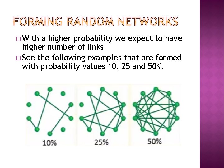
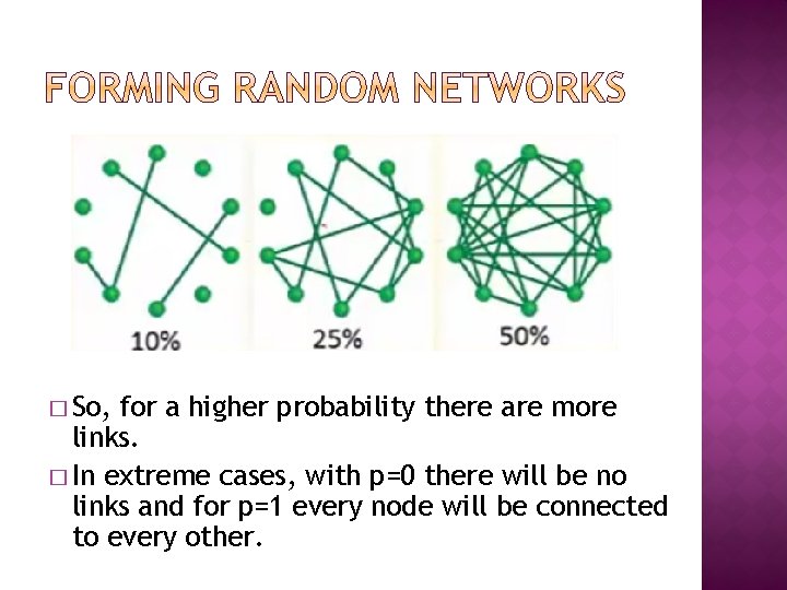
� With a higher probability we expect to have higher number of links. � See the following examples that are formed with probability values 10, 25 and 50%.

� So, for a higher probability there are more links. � In extreme cases, with p=0 there will be no links and for p=1 every node will be connected to every other.

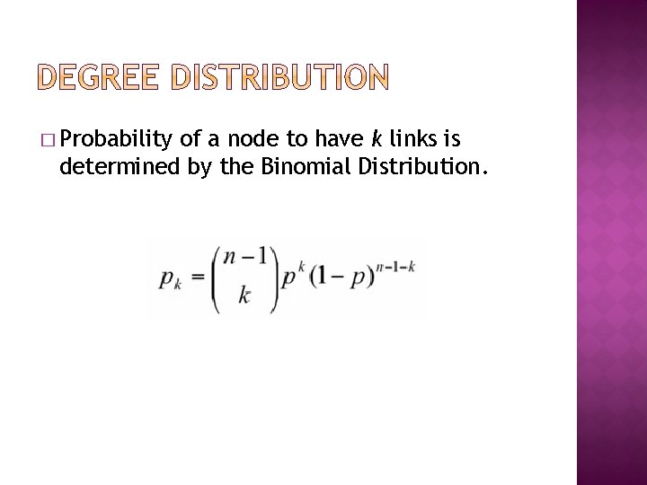
� Probability of a node to have k links is determined by the Binomial Distribution.

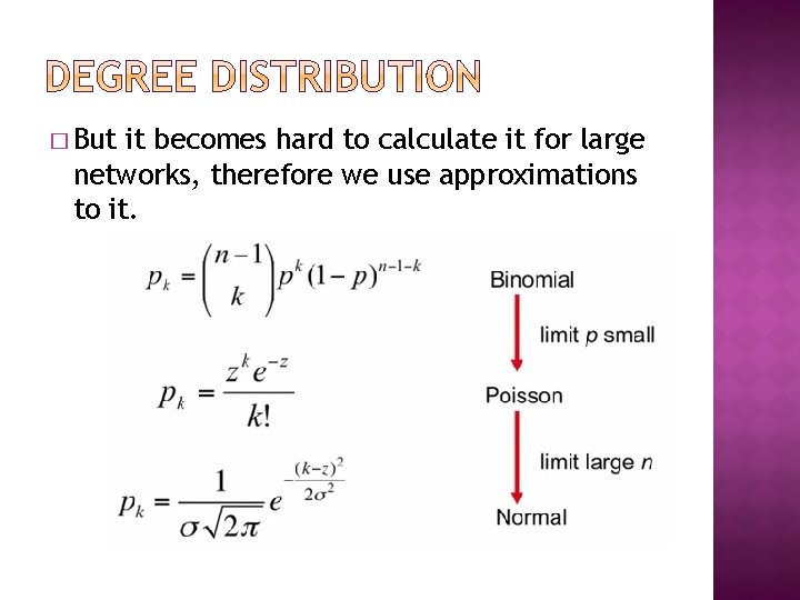
� But it becomes hard to calculate it for large networks, therefore we use approximations to it.

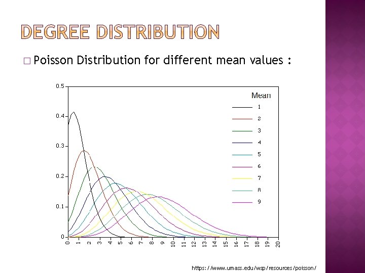
� Degree distribution will show us with what probability a node has k number of neighbors. � So, on the horizontal axes we have the degrees and on the vertical axes we have the probability to have that degree.

� Poisson Distribution for different mean values : https: //www. umass. edu/wsp/resources/poisson/

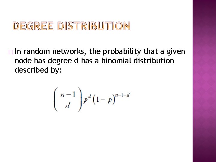
� In random networks, the probability that a given node has degree d has a binomial distribution described by:

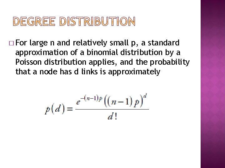
� For large n and relatively small p, a standard approximation of a binomial distribution by a Poisson distribution applies, and the probability that a node has d links is approximately

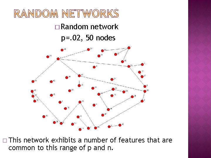
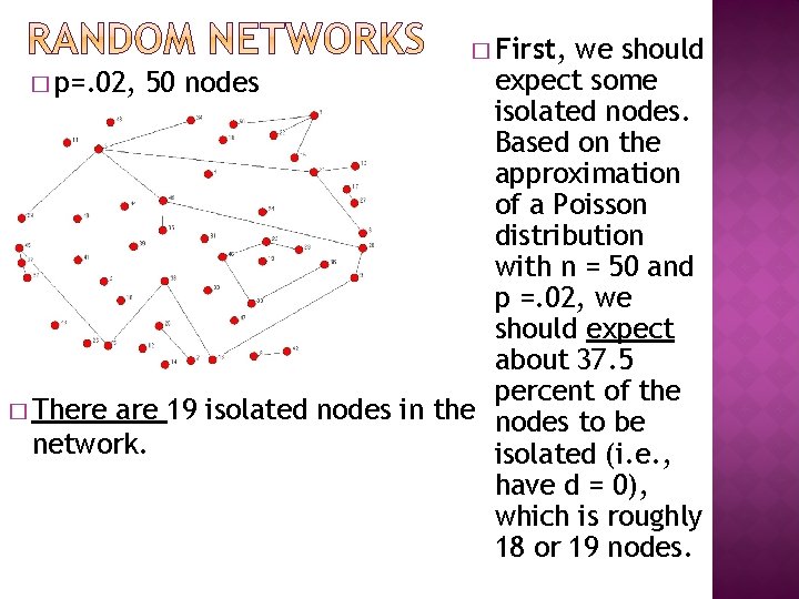
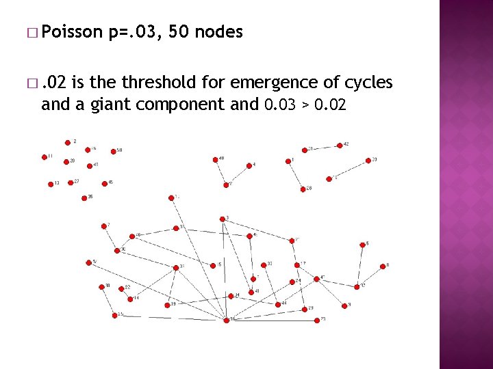
� Random network p=. 02, 50 nodes � This network exhibits a number of features that are common to this range of p and n.

� First, we should expect some � p=. 02, 50 nodes isolated nodes. Based on the approximation of a Poisson distribution with n = 50 and p =. 02, we should expect about 37. 5 percent of the � There are 19 isolated nodes in the nodes to be network. isolated (i. e. , have d = 0), which is roughly 18 or 19 nodes.

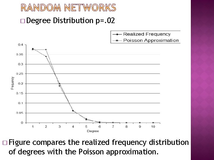
� Degree � Figure Distribution p=. 02 compares the realized frequency distribution of degrees with the Poisson approximation.

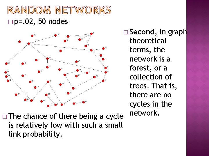
� p=. 02, 50 nodes � Second, in graph theoretical terms, the network is a forest, or a collection of trees. That is, there are no cycles in the network. � The chance of there being a cycle is relatively low with such a small link probability.

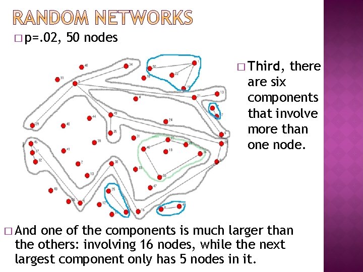
� p=. 02, 50 nodes � Third, there are six components that involve more than one node. � And one of the components is much larger than the others: involving 16 nodes, while the next largest component only has 5 nodes in it.

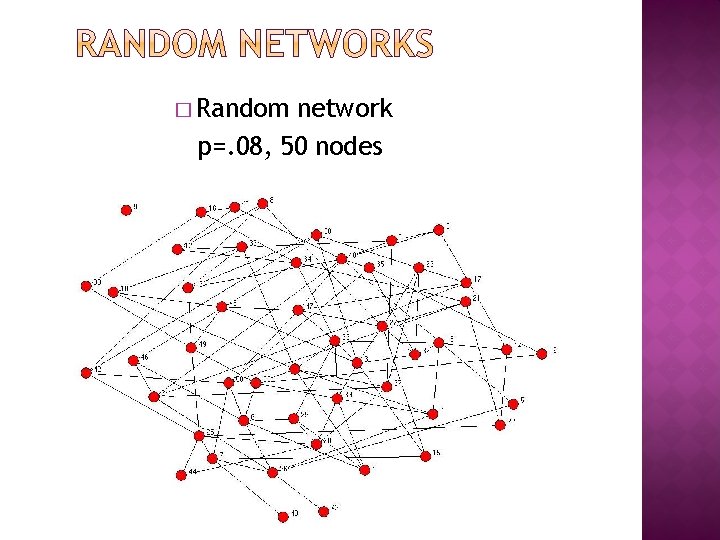
� Random network p=. 08, 50 nodes

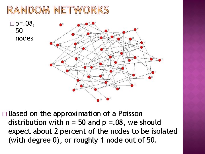
� p=. 08, 50 nodes � Based on the approximation of a Poisson distribution with n = 50 and p =. 08, we should expect about 2 percent of the nodes to be isolated (with degree 0), or roughly 1 node out of 50.

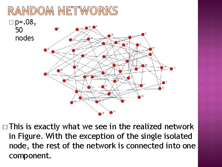
� p=. 08, 50 nodes � This is exactly what we see in the realized network in Figure. With the exception of the single isolated node, the rest of the network is connected into one component.

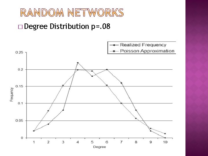
� Degree Distribution p=. 08

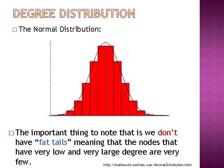
� The degree distribution of a random graph is a normal distribution, rather, the discrete counterpart of a bell curve, a binomial distribution

� The Normal Distribution: important thing to note that is we don’t have “fat tails” meaning that the nodes that have very low and very large degree are very few. http: //mathworld. wolfram. com/Normal. Distribution. html

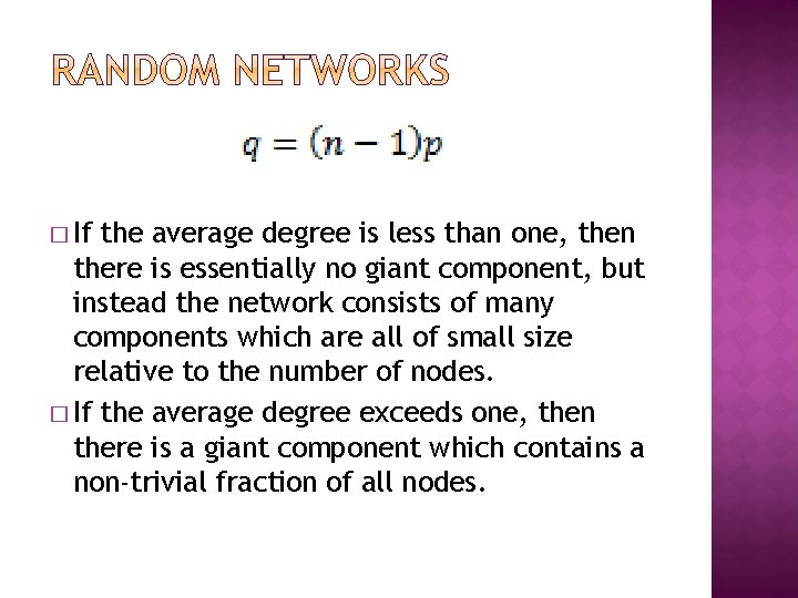
� We may note that the average degree of a node rises faster than the number of links (as every link added increases the degree of two nodes). � In fact, there is a marked difference in the structure of the resulting network depending on whether average degree is bigger or smaller than one.

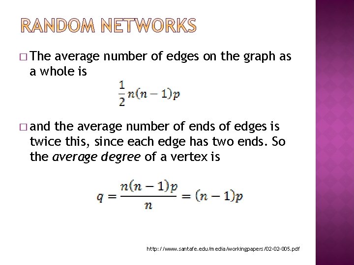
� The average number of edges on the graph as a whole is � and the average number of ends of edges is twice this, since each edge has two ends. So the average degree of a vertex is http: //www. santafe. edu/media/workingpapers/02‐ 005. pdf

� If the average degree is less than one, then there is essentially no giant component, but instead the network consists of many components which are all of small size relative to the number of nodes. � If the average degree exceeds one, then there is a giant component which contains a non‐trivial fraction of all nodes.

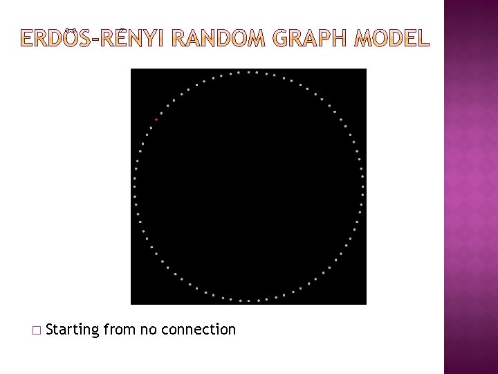
� Starting from no connection

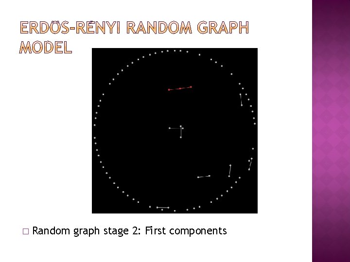
� Random graph stage 2: First components

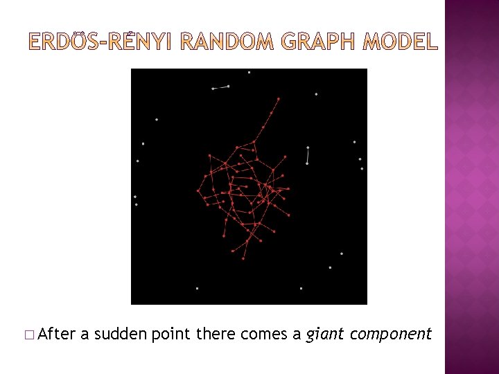
� After a sudden point there comes a giant component

� The sudden change in the component structure of many random graph processes is referred as the phase transition. � The value of the average degree for which this shift observed is called a critical point http: //edoc. hu‐berlin. de/dissertationen/seierstad‐taral‐ 2007‐ 06‐ 28/PDF/seierstad. pdf

� threshold function is a function that takes the value 1 if a specified function of the arguments exceeds a given threshold and 0 otherwise � Call this function as t(n) � A phase transition occurs at t(n) � This means that, in this particular case, with probability value greater than t(n) there will be a giant component and below we don’t have one.

� The term “giant component” refers to the unique largest component if there is one. � This may turn out to be a small component in some networks but we will generally be interested in giant components that involve non‐vanishing fractions of nodes, which will necessarily be “large” components. � Understanding giant components more generally is especially important as they play a central role in various problems of diffusion, � and a giant component gives an idea of the most nodes that one might possibly reach starting from a single node. Jackson(2008), p 139

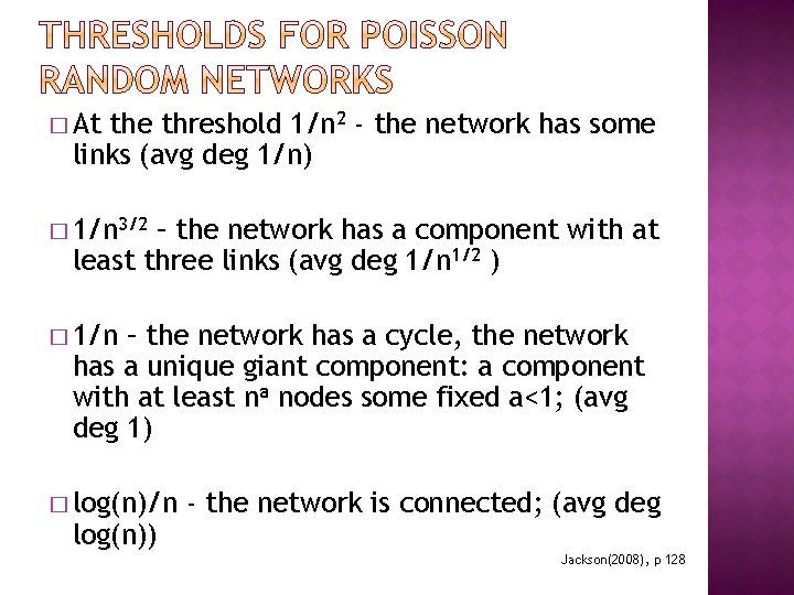
� At the threshold 1/n 2 ‐ the network has some links (avg deg 1/n) � 1/n 3/2 – the network has a component with at least three links (avg deg 1/n 1/2 ) � 1/n – the network has a cycle, the network has a unique giant component: a component with at least na nodes some fixed a<1; (avg deg 1) � log(n)/n log(n)) ‐ the network is connected; (avg deg Jackson(2008), p 128

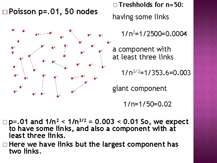
� Poisson p=. 01, 50 nodes � Treshholds for n=50: having some links 1/n 2=1/2500=0. 0004 a component with at least three links 1/n 3/2=1/353. 6=0. 003 giant component 1/n=1/50=0. 02 � p=. 01 and 1/n 2 < 1/n 3/2 = 0. 003 < 0. 01 So, we expect to have some links, and also a component with at least three links. � Here we have links but the largest component has two links.

� Poisson �. 02 p=. 03, 50 nodes is the threshold for emergence of cycles and a giant component and 0. 03 > 0. 02

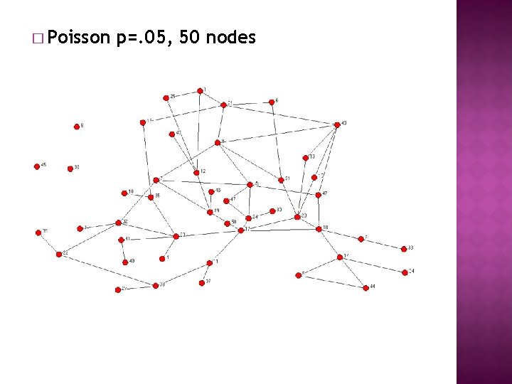
� Poisson p=. 05, 50 nodes

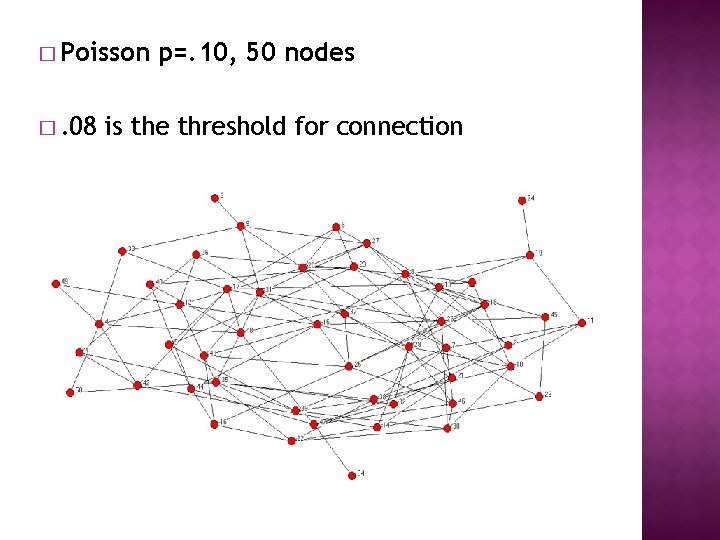
� Poisson �. 08 p=. 10, 50 nodes is the threshold for connection

� Growth of the Giant Component https: //www. youtube. com/watch? v=yjc. Vd. O 2 F 3 j 4 � Further notes https: //www. youtube. com/watch? v=89 mx. Odw Pfx. A

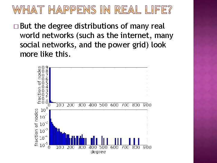
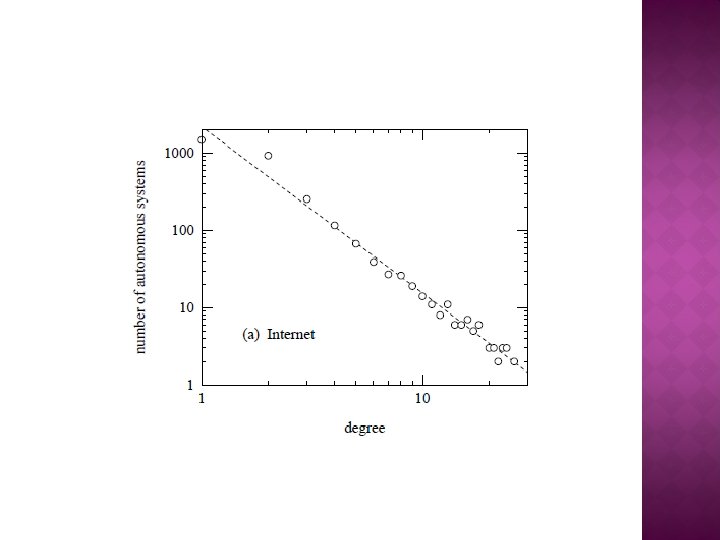
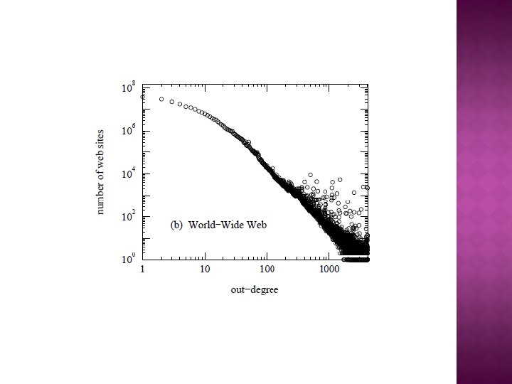
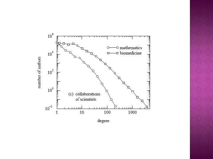
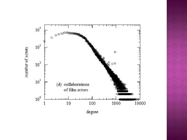
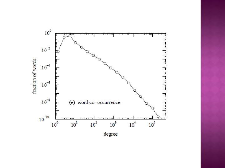
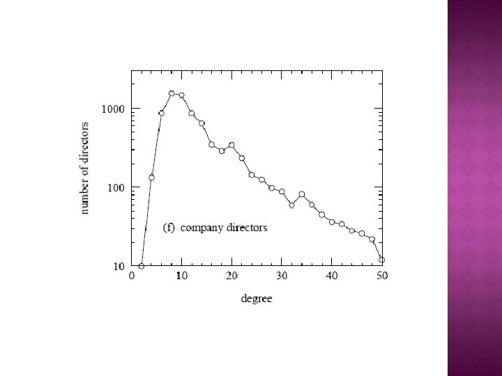
� But the degree distributions of many real world networks (such as the internet, many social networks, and the power grid) look more like this.

� This tells us that real world networks are not generated by the kind of process that generates a random graph.

� The average path length in random graphs is quite low, typically the log of the numbers of nodes. � That means that average path length grows much more slowly than the number of nodes. � This property is shared with social networks, as we shall see, and is crucial in characterizing so ‐called small world networks.

� In most of the real networks, despite of their often large size, there is a relatively short path between any two nodes. This feature is known as the small‐world (Boccaletti, 2006).

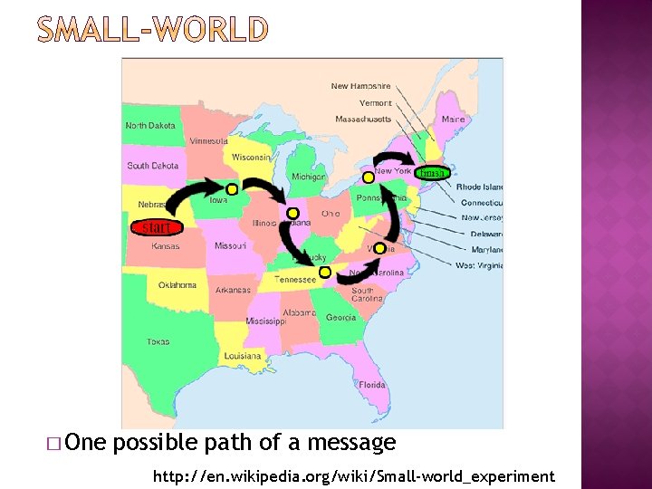
� In its first experiment, Milgram asked randomly selected people in Nebraska to send letters to a distant target individual in Boston, identified only by his name, occupation and rough location. � The letters could only be sent to someone whom the current holder knew by first name, and who was presumably closer to the final recipient. � 42 out of 160 letters reached to their targets.

� One possible path of a message http: //en. wikipedia. org/wiki/Small‐world_experiment

� Milgram kept track of the paths followed by the letters and of the demographic characteristics of their handlers. Although the common guess was that it might take hundreds of these steps for the letters to reach their final destination, Milgram’s surprising result was that the number of links needed to reach the target person had an average value of just six.

� Later John Guare used this idea on his play in 1991 which he named as “six degrees of separation”. � Afterwards Milgram’s idea was termed by this name. � Milgram showed that no matter how large of a society we are in, actually we are only few steps apart. So, we live in a “small world”.

� Consider another way around: � Organize a party with 100 guests who do not know each other. Offer them wine and cheese. They will soon start to chat. There will be groups of two or three. � Inform one of the guests about a wine in the unlabeled dark green bottles which is a rare twenty‐year‐old vintage port, that is much better than the labeled red wine. Ask the guest to share this information only with his/her new acquaintances.

� Guests will be bored talking to the same people and join to other groups. Now, two people that do not know each other directly may have a friend in common. � The news of a valuable wine will pass on to others through common friends of two strangers. � Will everyone be informed about the vintage wine before the end of the party?

� According to Paul Erdős and Alféd Rényi if each person gets to know at least one other guest, then soon everybody will be drinking the special wine. � It would take only thirty minutes to inform everyone in the room.

� Starting with a large number of isolated nodes, by randomly adding links between them, only little number of connections will result in some groups of nodes. � Continuing in this manner we obtain clusters of several nodes. And if we add enough links we end up with a giant cluster. So, most nodes will be a part of a single cluster in which every node is linked to the any other. � According to the random network theory as the average number of links per node increases beyond a critical number, the number of nodes left out of the giant cluster decreases exponentially.

� In mathematical terms, a small‐world network is a type of mathematical graph with special characteristics (see Milgram, 1967 and Watts, 1999 for details). It is widely used in recent studies of network modeling. � What makes it so attractive is its ability to describe the structure and dynamics of seemingly complex real‐life networks with simple explanations (Frommer and Pundoor, 2003).

� The small‐world nature of a graph comes from two things: its clustering coefficient and path length. � Such networks have small diameter and small average path lengths together with high clustering coefficients relative to networks generated by an independent random process (Jackson and Rogers, 2005).

� The clustering coefficient defines the extent to which nodes in the graph tend to merge so that there exists many arcs connecting each other in the group, but very few arcs leading out of the group. � Path length of a node is the shortest path lengths connecting that node in the graph to all other nodes. It measures the number of links that have to be formed in order to travel from one node to another. So, it describes the degree of separation or connectivity between nodes in the graph (Frommer and Pundoor, 2003).

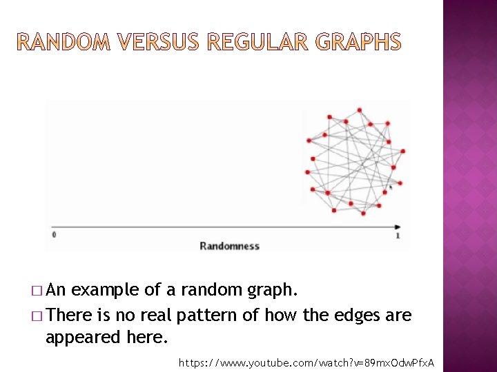
� An example of a random graph. � There is no real pattern of how the edges are appeared here. https: //www. youtube. com/watch? v=89 mx. Odw. Pfx. A

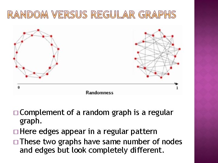
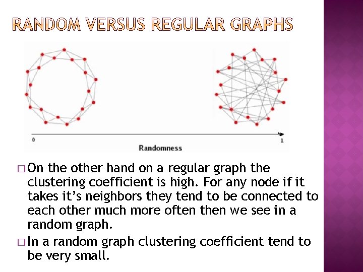
� Complement of a random graph is a regular graph. � Here edges appear in a regular pattern � These two graphs have same number of nodes and edges but look completely different.

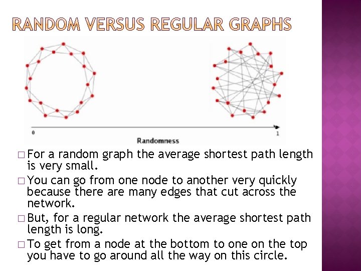
� For a random graph the average shortest path length is very small. � You can go from one node to another very quickly because there are many edges that cut across the network. � But, for a regular network the average shortest path length is long. � To get from a node at the bottom to one on the top you have to go around all the way on this circle.

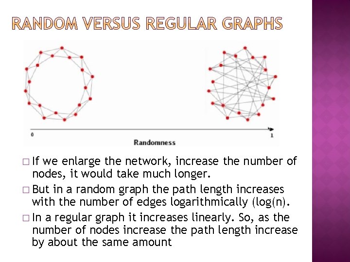
� If we enlarge the network, increase the number of nodes, it would take much longer. � But in a random graph the path length increases with the number of edges logarithmically (log(n). � In a regular graph it increases linearly. So, as the number of nodes increase the path length increase by about the same amount

� On the other hand on a regular graph the clustering coefficient is high. For any node if it takes it’s neighbors they tend to be connected to each other much more often then we see in a random graph. � In a random graph clustering coefficient tend to be very small.

� Remember the small‐world graphs have: Ø small average path lengths together with Ø high clustering coefficients (as random grapghs)

� So, random graphs have the first property but not the second � whereas the regular graphs have the second but not the first. � This problem is tried to be solved by some other modeling techniques.

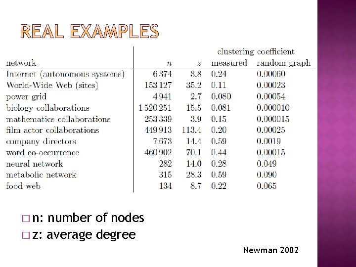
� n: number of nodes � z: average degree Newman 2002

� Internet: a graph of the fibre optic connections that comprise the Internet, at the level of so‐called autonomous systems. " An autonomous system is a group of computers within which data flow is handled autonomously, while data flow between groups is conveyed over the public Internet. Examples of autonomous systems might be the computers at a company, a university, or an Internet service provider. � World‐Wide Web: a graph of sites on the World‐Wide Web in which edges represent hyperlinks" connecting one site to another. A site in this case means a collection of pages residing on a server with a given name. Although hyperlinks are directional, their direction has been ignored in this calculation of the clustering coefficient.

� Power grid: a graph of the Western States electricity transmission grid in the United States. Vertices represent stations and substations; edges represent transmission lines. � Biology collaborations: a graph of collaborations between researchers working in biology and medicine. A collaboration between two scientists is defined in this case as co‐authorship of a paper that was catalogued in the Medline bibliographic database between 1995 and 1999 inclusive. � Mathematics collaborations: a similar collaboration graph for mathematicians, derived from the archives of Mathematical Reviews.

� Film actor collaborations: a graph of collaborations between film actors, where a collaboration means that the two actors in question have appeared in a film together. The data are from the Internet Movie Database. � Company directors: a collaboration graph of the directors of companies in the Fortune 1000 for 1999. (The Fortune 1000 is the 1000 US companies with the highest revenues during the year in question. ) Collaboration in this case means that two directors served on the board of a Fortune 1000 company together. � Word co‐occurrences: a graph in which the vertices represent words in the English language, and an edge refers that the vertices it connects frequently occur in adjacent positions in sentences.

� Neural network: a graph of the neural network of the worm C. Elegans. � Metabolic network: a graph of interactions forming a part of the energy generation and small building block synthesis metabolism of the bacterium E. Coli. Vertices represent substrates and products, and edges represent interactions. � Food web: the food web of predator‐prey interactions between species in Ythan Estuary, a marine estuary near Aberdeen, Scotland. Like the links in the World‐Wide Web graph, the directed nature of the interactions in this food web have been neglected for the purposes of calculating the clustering coefficient.