Lecture 3 Simple Keynesian Model National Income Determination

Lecture 3: Simple Keynesian Model National Income Determination Three-Sector National Income Model 1

Outline Three-Sector Model ◦ Output-Expenditure Approach: Equilibrium National Income Ye ◦ Injection-Withdrawal Approach: Equilibrium National Income Ye Fiscal Policy 2

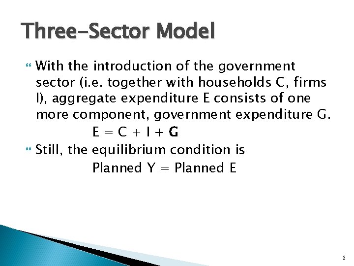
Three-Sector Model With the introduction of the government sector (i. e. together with households C, firms I), aggregate expenditure E consists of one more component, government expenditure G. E=C+I+G Still, the equilibrium condition is Planned Y = Planned E 3

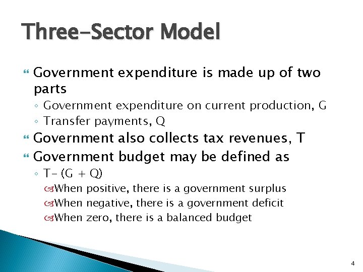
Three-Sector Model Government expenditure is made up of two parts ◦ Government expenditure on current production, G ◦ Transfer payments, Q Government also collects tax revenues, T Government budget may be defined as ◦ T- (G + Q) When positive, there is a government surplus When negative, there is a government deficit When zero, there is a balanced budget 4

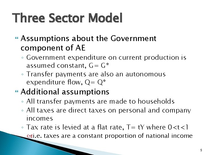
Three Sector Model Assumptions about the Government component of AE ◦ Government expenditure on current production is assumed constant, G= G* ◦ Transfer payments are also an autonomous expenditure flow, Q= Q* Additional assumptions ◦ All transfer payments are made to households ◦ All taxes are direct taxes on personal and company incomes ◦ Tax rate is levied at a flat rate, T= t. Y where 0<t<1 i. e. taxes are a constant proportion of national income 5

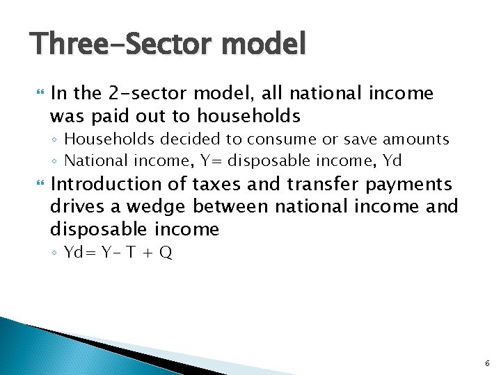
Three-Sector model In the 2 -sector model, all national income was paid out to households ◦ Households decided to consume or save amounts ◦ National income, Y= disposable income, Yd Introduction of taxes and transfer payments drives a wedge between national income and disposable income ◦ Yd= Y- T + Q 6

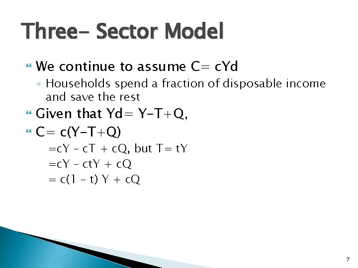
Three- Sector Model We continue to assume C= c. Yd ◦ Households spend a fraction of disposable income and save the rest Given that Yd= Y-T+Q, C= c(Y-T+Q) =c. Y – c. T + c. Q, but T= t. Y =c. Y – ct. Y + c. Q = c(1 – t) Y + c. Q 7

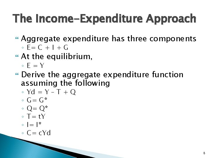
The Income-Expenditure Approach Aggregate expenditure has three components ◦ E= C + I + G At the equilibrium, ◦ E=Y Derive the aggregate expenditure function assuming the following ◦ ◦ ◦ Yd = Y – T + Q G= G* Q= Q* T= t. Y I= I* C= c. Yd 8

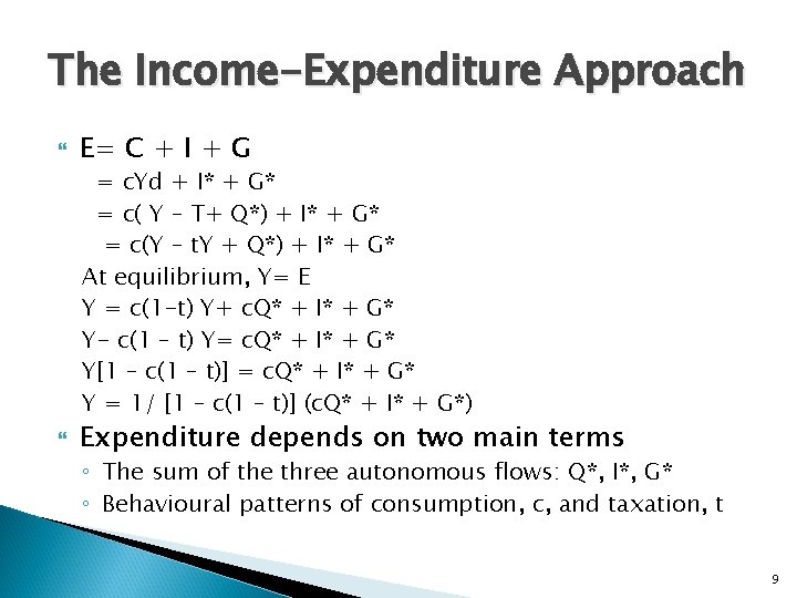
The Income-Expenditure Approach E= C + I + G = c. Yd + I* + G* = c( Y – T+ Q*) + I* + G* = c(Y – t. Y + Q*) + I* + G* At equilibrium, Y= E Y = c(1 -t) Y+ c. Q* + I* + G* Y- c(1 – t) Y= c. Q* + I* + G* Y[1 – c(1 – t)] = c. Q* + I* + G* Y = 1/ [1 – c(1 – t)] (c. Q* + I* + G*) Expenditure depends on two main terms ◦ The sum of the three autonomous flows: Q*, I*, G* ◦ Behavioural patterns of consumption, c, and taxation, t 9

Changes in Equilibrium Income What is the effect of changes in autonomous expenditure flows and the tax rate, t, on national income? 10

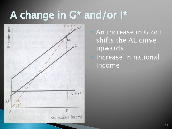
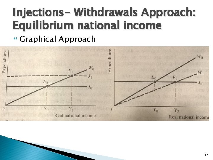
A change in G* and/or I* An increase in G or I shifts the AE curve upwards Increase in national income 11

A change in transfer payments An increase in transfer payments will also increase national income ◦ How? However, an extra Ghc 1 spent on final government expenditure, G, increases national income by more than Ghc 1 spent on transfer payment, Q. ◦ Why? 12

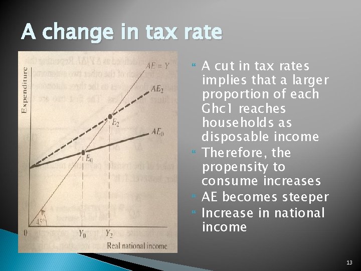
A change in tax rate A cut in tax rates implies that a larger proportion of each Ghc 1 reaches households as disposable income Therefore, the propensity to consume increases AE becomes steeper Increase in national income 13

The Multiplier How large is the change in national income from a given change in autonomous expenditure? To determine this, we need to solve the following algebraically: ◦ Ye/ I ◦ Ye/ G ◦ Ye/ Q 14

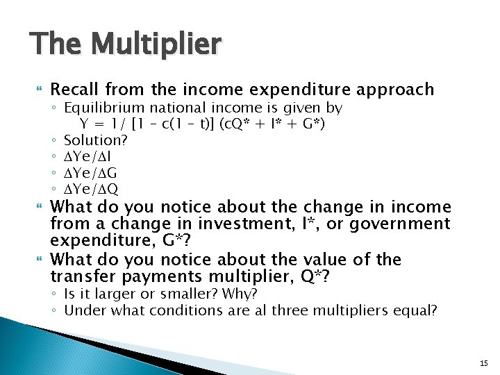
The Multiplier Recall from the income expenditure approach ◦ Equilibrium national income is given by Y = 1/ [1 – c(1 – t)] (c. Q* + I* + G*) ◦ Solution? ◦ Ye/ I ◦ Ye/ G ◦ Ye/ Q What do you notice about the change in income from a change in investment, I*, or government expenditure, G*? What do you notice about the value of the transfer payments multiplier, Q*? ◦ Is it larger or smaller? Why? ◦ Under what conditions are al three multipliers equal? 15

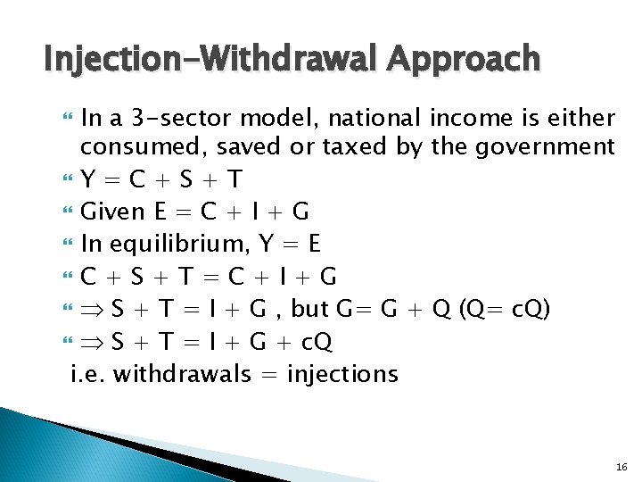
Injection-Withdrawal Approach In a 3 -sector model, national income is either consumed, saved or taxed by the government Y = C + S + T Given E = C + I + G In equilibrium, Y = E C + S + T = C + I + G S + T = I + G , but G= G + Q (Q= c. Q) S + T = I + G + c. Q i. e. withdrawals = injections 16

Injections- Withdrawals Approach: Equilibrium national income Graphical Approach 17

Injections- Withdrawals Approach: Equilibrium national income Graphical Approach ◦ An increase in any component of aggregate expenditure shifts the injections curve upwards And vice versa ◦ A fall in the tax rate increases the amount of disposable income, and the propensity for increased consumption This is illustrated by a flatter (i. e. smaller value of t) withdrawals curve, leading to increased equilibrium national income 18

Injections- Withdrawals Approach: Equilibrium national income An algebraic approach ◦ We define savings, S= s(Y- T) ◦ i. e. the part of national income that is saved ◦ Other assumptions ◦ ◦ ◦ T= t. Y Q= Q* I= I* G= G* At the equilibrium, Withdrawals = Injections Withdrawals = s(1 - t)Y + t. Y = Y[s(1 - t) + t] Injections = I* + G* + c. Q* At the equilibrium, Y =1/ [s(1 - t) + t] x (I* + G* + c. Q*) Is this the same equilibrium as obtained under the income-expenditure approach? Derive the multipliers for investment and government expenditures, and transfer payments. 19

Limitation of the Simple Keynesian model Y = Multiplier* G* There are several problems with this method of analysis, i. e. , Y may be less ◦ Sources of financing G* ◦ Effects on private investment I* ◦ Productivity of government projects 20

The Problems of the Simple Keynesian Multiplier k E Sources of financing G’ Increasing Tax ◦ will exert a contractionary effect on the economy Increasing Money Supply ◦ will generate an inflationary pressure Prices assumed constant Increasing Debt/ Private sector borrowing ◦ will increase the demand for loanable fund as well as interest rate affect private investment 21

The Problems of the Simple Keynesian Multiplier k E Effects on Private Investment I’ Private investment may be crowded out when government increases its expenditure ◦ It is questionable that the government can really produce something which is desired by the consumers Besides, government investment projects are usually less productive than private investment projects 22

The Problems of the Simple Keynesian Multiplier k E Productivity of Government Projects Government projects may not yield a rate of return (MEC / MEI) exceeding the market interest rate. 23

Take- Home Assignment Using the mechanistic Keynes Theory of National Income, explain the causes and solutions to the Great Depression of 1929. 24

Next Class Money and its Functions The origin of money Modern money and definition of monetary aggregates Commercial Banks and Money Creation The Central Bank and its functions 25