Lecture 3 Review Measures of central tendency location

Lecture 3

Review: Measures of central tendency (location) Which measures of location do you know + what is their meaning? How we can find the median, if the number of values is odd? How we can find the median, if the number of values is even? Which measure of location is the “best”?

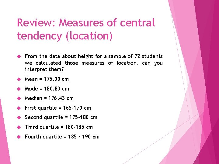
Review: Measures of central tendency (location) From the data about height for a sample of 72 students we calculated those measures of location, can you interpret them? Mean = 175. 00 cm Mode = 180. 83 cm Median = 176. 43 cm First quartile = 165 -170 cm Second quartile = 175 -180 cm Third quartile = 180 -185 cm Fourth quartile = 185 – 190 cm

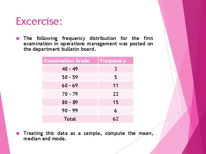
Excercise: The following frequency distribution for the first examination in operations management was posted on the department bulletin board. Examination Grade Frequency 40 – 49 3 50 – 59 5 60 – 69 11 70 – 79 22 80 – 89 15 90 – 99 6 Total 62 Treating this data as a sample, compute the mean, median and mode.

Describing Data: Numerical 2. part Figures won´t lie, but liars will figure

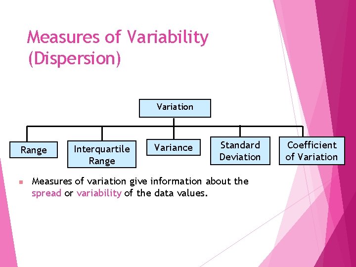
Measures of Variability (Dispersion) Variation Range n Interquartile Range Variance Standard Deviation Measures of variation give information about the spread or variability of the data values. Coefficient of Variation

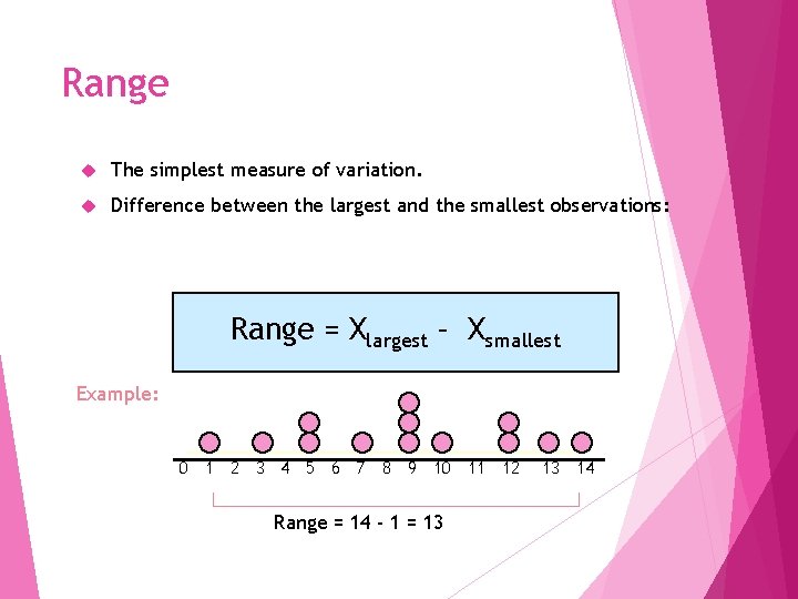
Range The simplest measure of variation. Difference between the largest and the smallest observations: Range = Xlargest – Xsmallest Example: 0 1 2 3 4 5 6 7 8 9 10 11 12 Range = 14 - 1 = 13 13 14

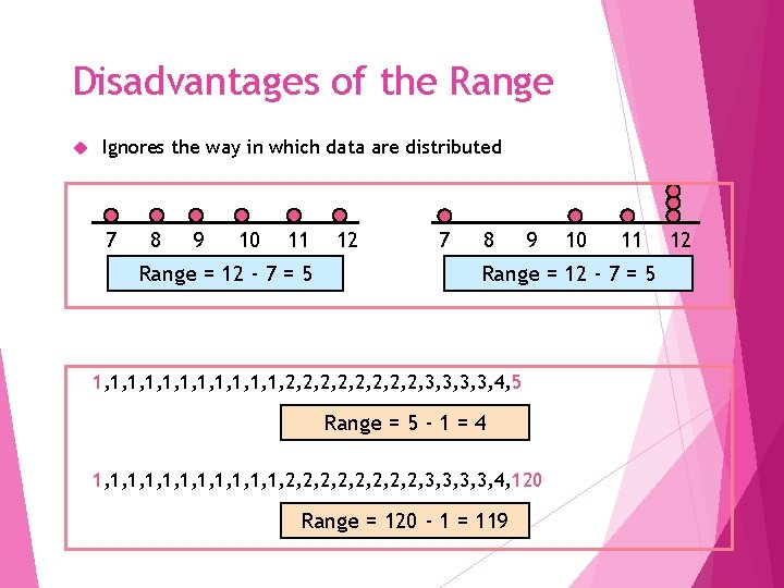
Disadvantages of the Range Ignores the way in which data are distributed 7 8 9 10 11 Range = 12 - 7 = 5 12 7 8 9 10 11 Range = 12 - 7 = 5 1, 1, 1, 2, 2, 3, 3, 4, 5 Range = 5 - 1 = 4 1, 1, 1, 2, 2, 3, 3, 4, 120 Range = 120 - 1 = 119 12

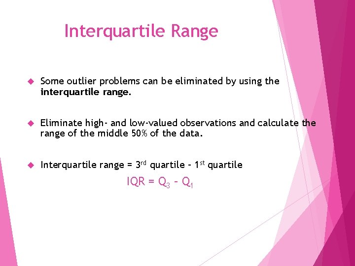
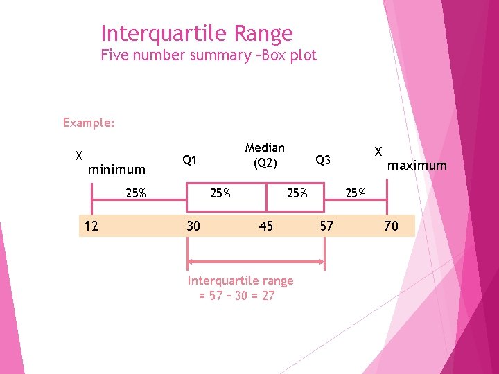
Interquartile Range Some outlier problems can be eliminated by using the interquartile range. Eliminate high- and low-valued observations and calculate the range of the middle 50% of the data. Interquartile range = 3 rd quartile – 1 st quartile IQR = Q 3 – Q 1

Five number summary In a five number summary, the following five numbers are used to summarize the data: 1. Smallest value 2. First quartile 3. Median 4. Third quartile 5. Largest value Those five values are usually shown in a graph, called Box plot.

Box plot The box plot is a relatively recent development in the area of graphical summaries of data. Key to the development of a box plot is the computation of the median and the quartiles, Q 1 and Q 3. The interquartile range, IQR = Q 3 – Q 1, is also used. The steps used to construct the box plot are: 1. A box is drawn with the ends of the box located at the first and third quartiles (this box contains the middle 50% of the data). 2. A vertical line is drawn in the box at the location of the median. Thus the median line divides the data into two equals parts. 3. The horizontal lines are called whiskers. The whiskers are drawn from the ends of the box to the smallest and largest data values.

Interquartile Range Five number summary –Box plot Example: X minimum Q 1 25% 12 Median (Q 2) 25% 30 X Q 3 25% 45 Interquartile range = 57 – 30 = 27 maximum 25% 57 70

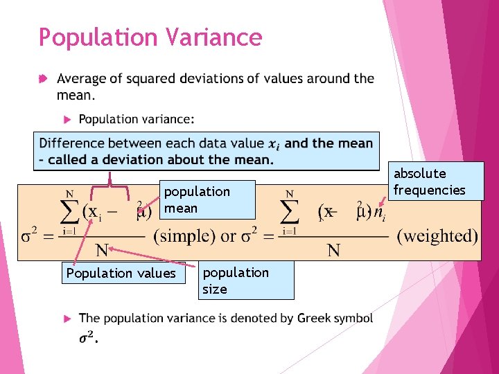
Population Variance population mean Population values population size absolute frequencies

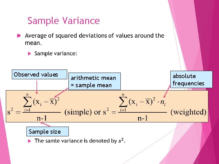
Sample Variance Observed values Sample size arithmetic mean = sample mean absolute frequencies

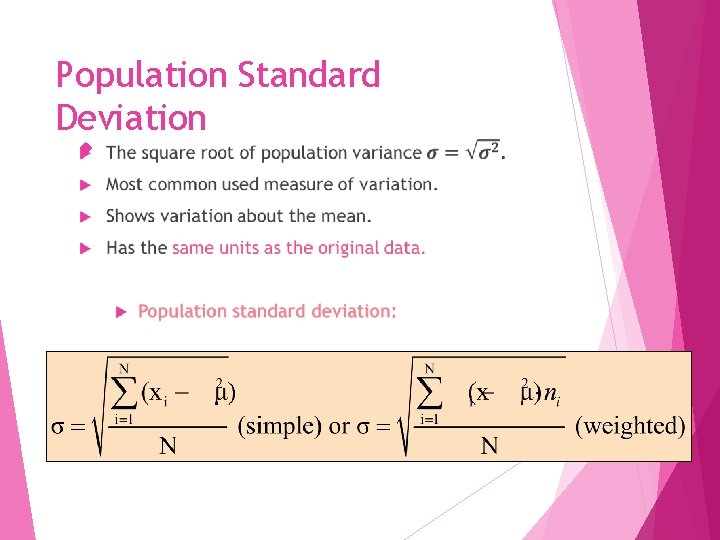
Population Standard Deviation

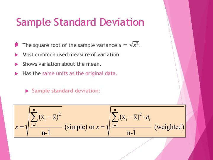
Sample Standard Deviation

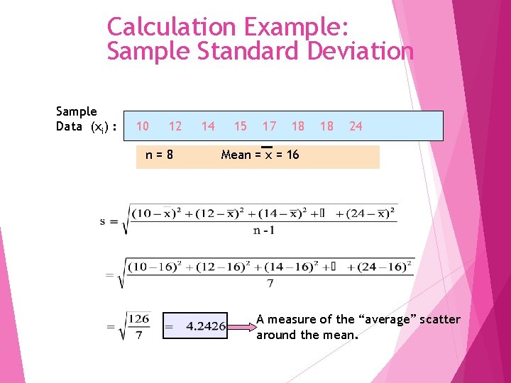
Calculation Example: Sample Standard Deviation Sample Data (xi) : 10 12 n=8 14 15 17 18 18 24 Mean = x = 16 A measure of the “average” scatter around the mean.

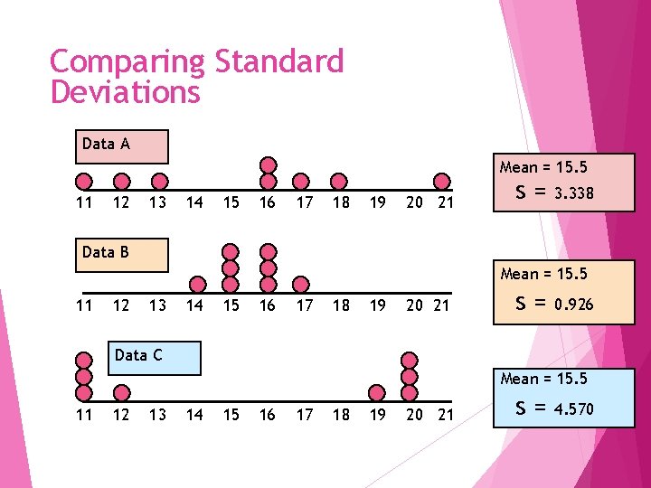
Comparing Standard Deviations Data A Mean = 15. 5 11 12 13 14 15 16 17 18 19 20 21 s= 3. 338 Data B Mean = 15. 5 11 12 13 14 15 16 17 18 19 20 21 s= 0. 926 Data C Mean = 15. 5 11 12 13 14 15 16 17 18 19 20 21 s= 4. 570

Advantages of Variance and Standard Deviation Each value in the data set is used in the calculation. Values far from the mean are given extra weight (because deviations from the mean are squared).

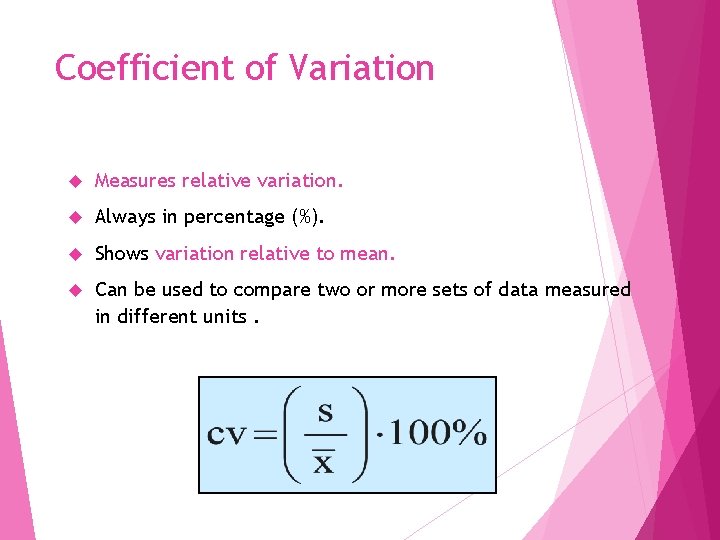
Coefficient of Variation Measures relative variation. Always in percentage (%). Shows variation relative to mean. Can be used to compare two or more sets of data measured in different units.

Excercise: 1. Consider the sample of size 5 with data values as follows: 10 20 12 17 16 Compute the variance and standard deviation. 2. Data on selling prices of automobiles were provided in U. S. News & World Report. Data in thousands of dollars are shown below: 5. 0 4. 4 5. 6 10. 4 9. 4 7. 0 9. 3 4. 5 4. 2 7. 7 11. 2 a) Compute the mean and median. b) Compute the range, interquartile range, and standard deviation.

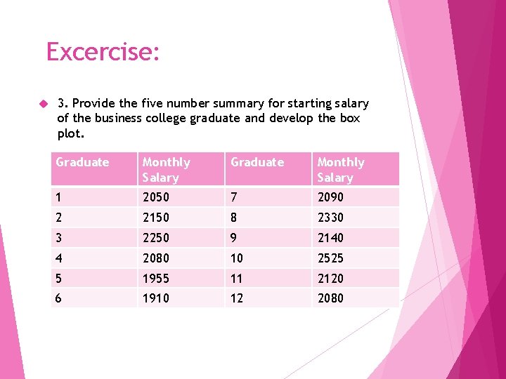
Excercise: 3. Provide the five number summary for starting salary of the business college graduate and develop the box plot. Graduate Monthly Salary 1 2050 7 2090 2 2150 8 2330 3 2250 9 2140 4 2080 10 2525 5 1955 11 2120 6 1910 12 2080

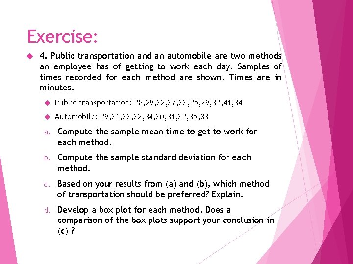
Exercise: 4. Public transportation and an automobile are two methods an employee has of getting to work each day. Samples of times recorded for each method are shown. Times are in minutes. Public transportation: 28, 29, 32, 37, 33, 25, 29, 32, 41, 34 Automobile: 29, 31, 33, 32, 34, 30, 31, 32, 35, 33 a. Compute the sample mean time to get to work for each method. b. Compute the sample standard deviation for each method. c. Based on your results from (a) and (b), which method of transportation should be preferred? Explain. d. Develop a box plot for each method. Does a comparison of the box plots support your conclusion in (c) ?

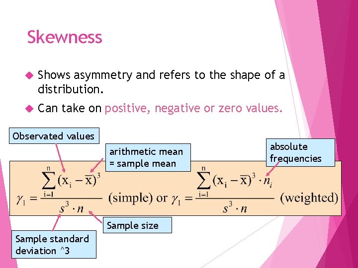
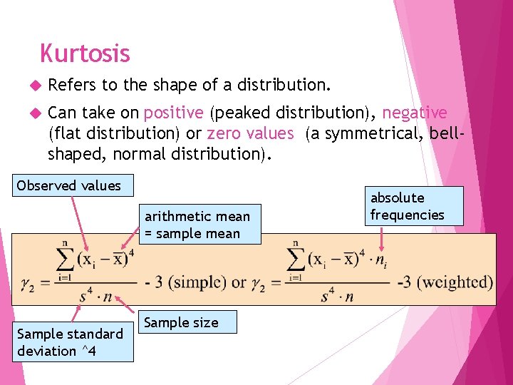
Skewness Shows asymmetry and refers to the shape of a distribution. Can take on positive, negative or zero values. Observated values arithmetic mean = sample mean Sample size Sample standard deviation ^3 absolute frequencies

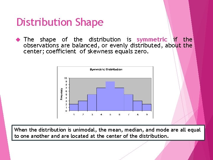
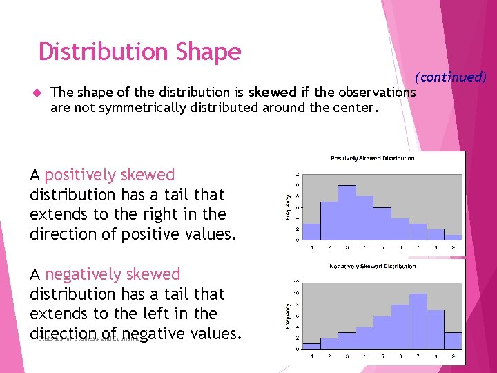
Distribution Shape The shape of the distribution is symmetric if the observations are balanced, or evenly distributed, about the center; coefficient of skewness equals zero. When the distribution is unimodal, the mean, median, and mode are all equal to one another and are located at the center of the distribution.

Distribution Shape (continued) The shape of the distribution is skewed if the observations are not symmetrically distributed around the center. A positively skewed distribution has a tail that extends to the right in the direction of positive values. A negatively skewed distribution has a tail that extends to the left in the direction of negative values. Statistics for Business and Economics Chap 3 -26

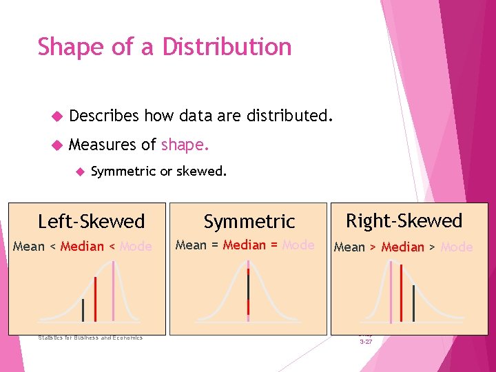
Shape of a Distribution Describes how data are distributed. Measures of shape. Symmetric or skewed. Left-Skewed Mean < Median < Mode Statistics for Business and Economics Symmetric Mean = Median = Mode Right-Skewed Mean > Median > Mode Chap 3 -27

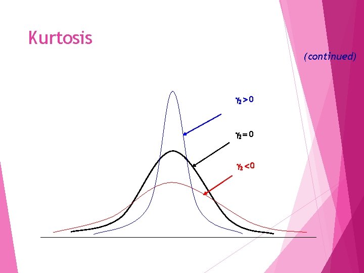
Kurtosis Refers to the shape of a distribution. Can take on positive (peaked distribution), negative (flat distribution) or zero values (a symmetrical, bellshaped, normal distribution). Observed values arithmetic mean = sample mean Sample standard deviation ^4 Sample size absolute frequencies

Kurtosis (continued) g 2 > 0 g 2 = 0 g 2 < 0

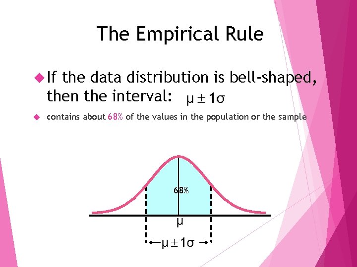
The Empirical Rule If the data distribution is bell-shaped, then the interval: contains about 68% of the values in the population or the sample 68%

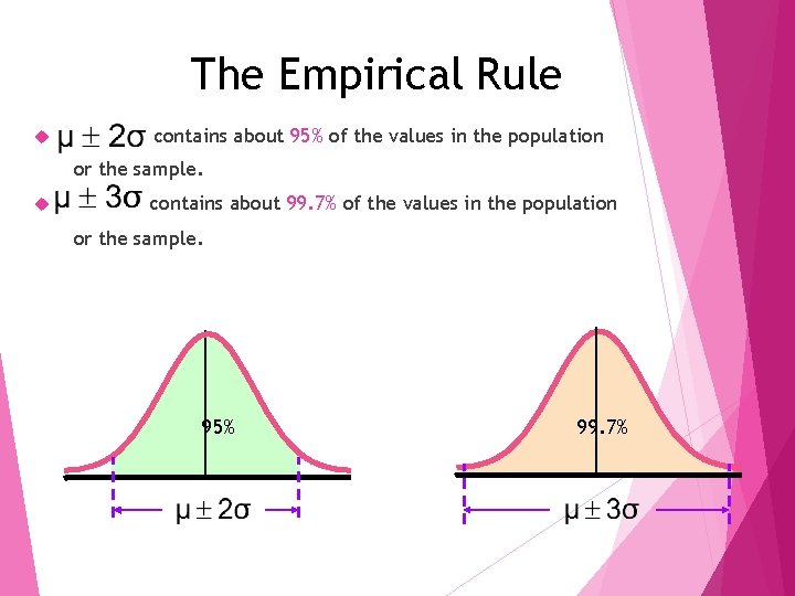
The Empirical Rule contains about 95% of the values in the population or the sample. contains about 99. 7% of the values in the population or the sample. 95% 99. 7%

Excercise: 1. Data that have a bell-shaped distribution have a mean of 30 and standard deviation of 5. Use the empirical rule to determine the proportion, or percentage, of data within each of the following ranges: 20 to 40 b. 15 to 45 c. 25 to 35 2. The IQ scores have a bell-shaped distribution with a mean of 100 and the standard deviation of 15. a. What percentage of the population should have an IQ score between 85 and 115? b. What percentage of the population should have an IQ score between 70 and 130? C. What percentage of the population should have an IQ score of more than 130?

Statistics for Business and Economics, 6 e © 2007 Pearson Education, Inc. Chap 3 -33

Using Microsoft Excel Simple Descriptive Statistics can be obtained from Microsoft® Excel Use menu choice: Data Tab / Data analysis / Descriptive statistics Enter details in dialog box.

Using Microsoft Excel (continued) Enter dialog box details Check box for summary statistics Click OK

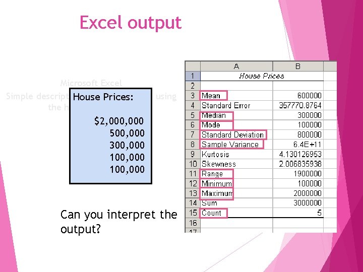
Excel output Microsoft Excel Simple descriptive statistics output, using House Prices: the house price data: $2, 000 500, 000 300, 000 100, 000 Can you interpret the output?

Thank you! Have a nice day!