Lecture 3 Region Based Vision Dr Carole Twining

Lecture 3: Region Based Vision Dr Carole Twining Thursday 18 th March 1: 00 pm – 1: 50 pm

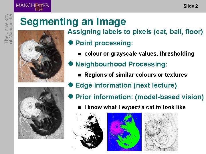
Slide 2 Segmenting an Image Assigning labels to pixels (cat, ball, floor) ● Point processing: n colour or grayscale values, thresholding ● Neighbourhood Processing: n Regions of similar colours or textures ● Edge information (next lecture) ● Prior information: (model-based vision) n I know what I expect a cat to look like

Slide 3 Overview ● Automatic threshold detection n Earlier, we did by inspection/guessing ● Multi-Spectral segmentation n satellite and medical image data ● Split and Merge n Hierarchical, region-based approach ● Relaxation labelling n probabilistic, learning approach ● Segmentation as optimisation

Automatic Threshold Selection

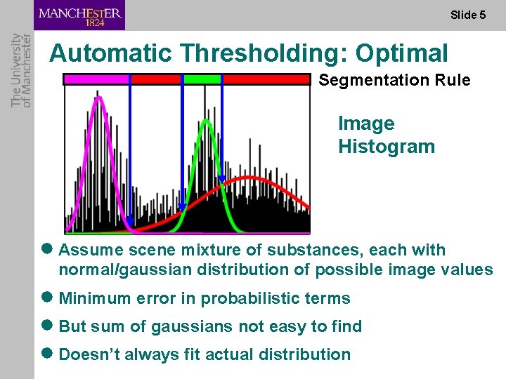
Slide 5 Automatic Thresholding: Optimal Segmentation Rule Image Histogram ● Assume scene mixture of substances, each with normal/gaussian distribution of possible image values ● Minimum error in probabilistic terms ● But sum of gaussians not easy to find ● Doesn’t always fit actual distribution

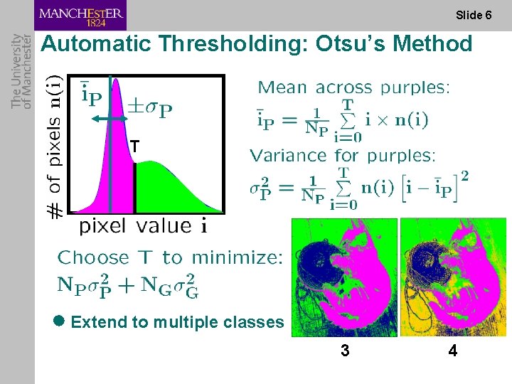
Slide 6 Automatic Thresholding: Otsu’s Method T ● Extend to multiple classes 3 4

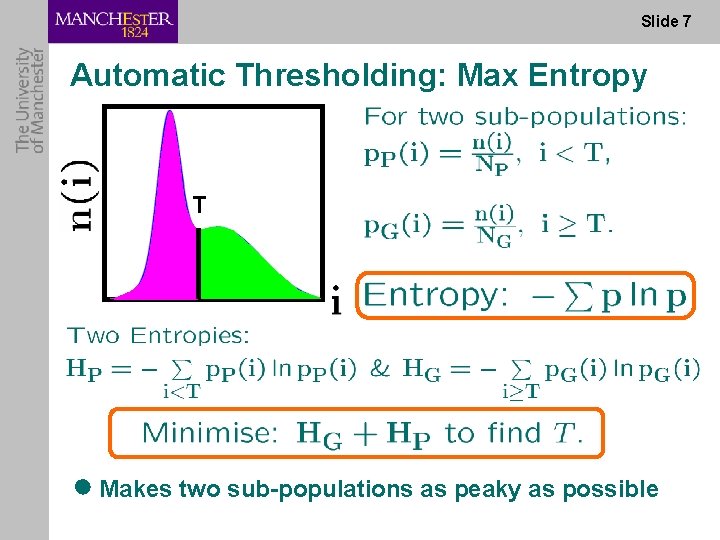
Slide 7 Automatic Thresholding: Max Entropy T ● Makes two sub-populations as peaky as possible

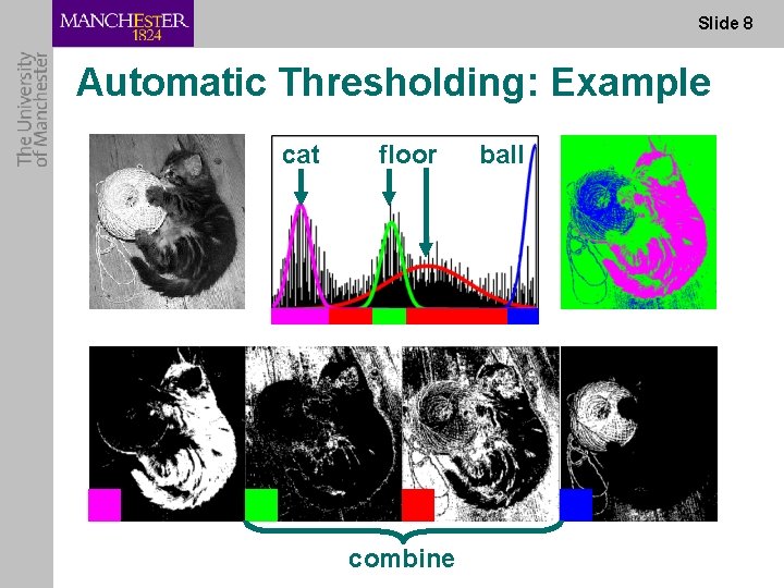
Slide 8 Automatic Thresholding: Example cat floor combine ball

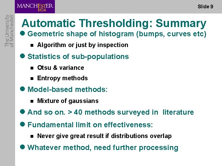
Slide 9 Automatic Thresholding: Summary ● Geometric shape of histogram (bumps, curves etc) n Algorithm or just by inspection ● Statistics of sub-populations n Otsu & variance n Entropy methods ● Model-based methods: n Mixture of gaussians ● And so on. > 40 methods surveyed in literature ● Fundamental limit on effectiveness: n Never give great result if distributions overlap ● Whatever method, need further processing

Multi-Spectral Segmentation

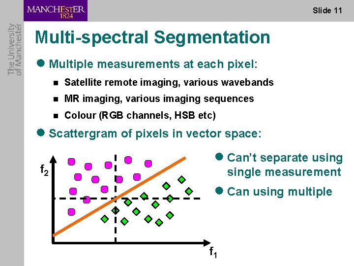
Slide 11 Multi-spectral Segmentation ● Multiple measurements at each pixel: n Satellite remote imaging, various wavebands n MR imaging, various imaging sequences n Colour (RGB channels, HSB etc) ● Scattergram of pixels in vector space: ● Can’t separate using f 2 single measurement ● Can using multiple f 1

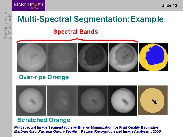
Slide 12 Multi-Spectral Segmentation: Example Spectral Bands Over-ripe Orange Scratched Orange Multispectral Image Segmentation by Energy Minimization for Fruit Quality Estimation: Martínez-Usó, Pla, and García-Sevilla, Pattern Recognition and Image Analysis , 2005

Split and Merge

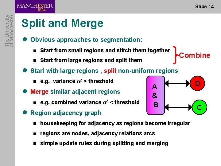
Slide 14 Split and Merge ● Obvious approaches to segmentation: n Start from small regions and stitch them together n Start from large regions and split them Combine ● Start with large regions , split non-uniform regions n e. g. variance 2 > threshold ● Merge similar adjacent regions n e. g. combined variance 2 < threshold ● Region adjacency graph A A & B B n housekeeping for adjacency as regions become irregular n regions are nodes, adjacency relations arcs n simple update rules during splitting and merging D C

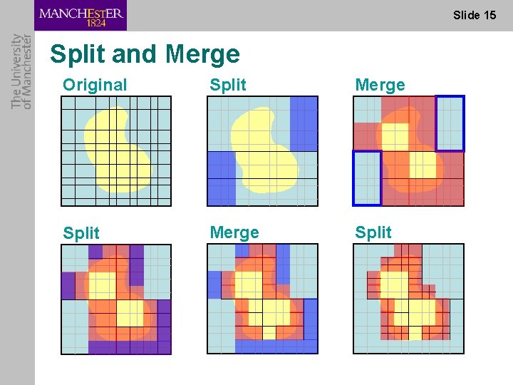
Slide 15 Split and Merge Original Split Merge Split

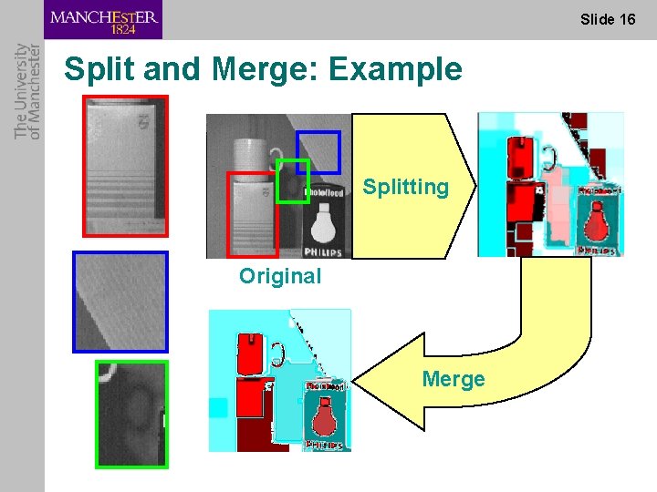
Slide 16 Split and Merge: Example Splitting Original Merge

Relaxation Labelling

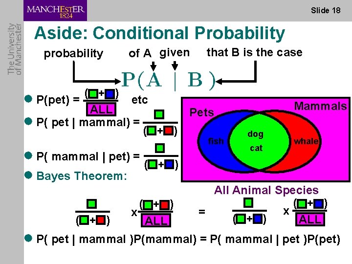
Slide 18 Aside: Conditional Probability probability of A given ( + ) ● P(pet) = etc ALL ● P( pet | mammal) = ( + ) ● P( mammal | pet) = ( + ) ● Bayes Theorem: ( + ) x ALL that B is the case Mammals Pets fish dog cat whale All Animal Species ( + ) x = ( + ) ALL ● P( pet | mammal )P(mammal) = P( mammal | pet )P(pet)

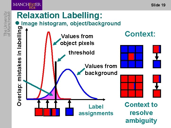
Slide 19 Overlap: mistakes in labelling Relaxation Labelling: ● Image histogram, object/background Values from object pixels Context: threshold Values from background Label assignments Context to resolve ambiguity

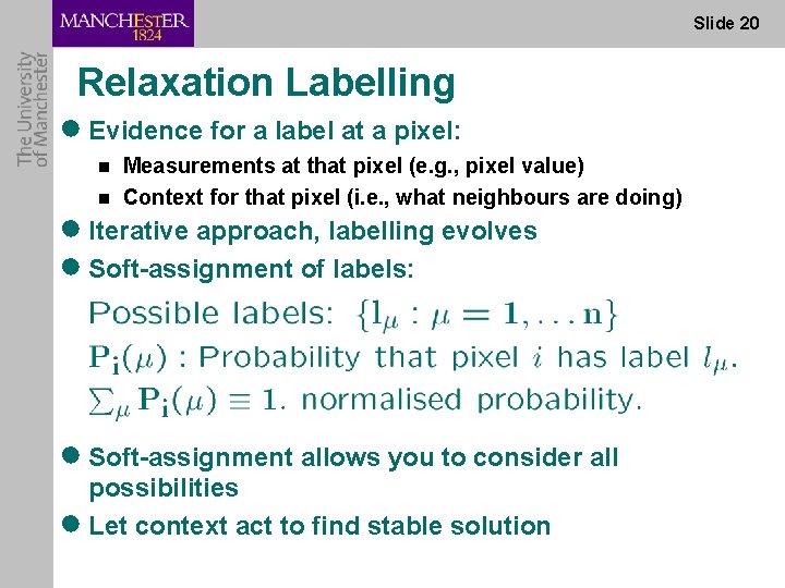
Slide 20 Relaxation Labelling ● Evidence for a label at a pixel: n n Measurements at that pixel (e. g. , pixel value) Context for that pixel (i. e. , what neighbours are doing) ● Iterative approach, labelling evolves ● Soft-assignment of labels: ● Soft-assignment allows you to consider all possibilities ● Let context act to find stable solution

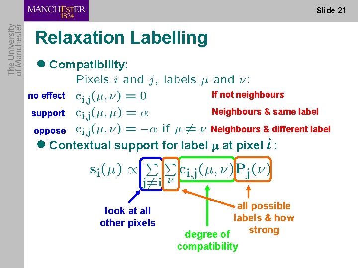
Slide 21 Relaxation Labelling ● Compatibility: If not neighbours no effect support Neighbours & same label oppose Neighbours & different label ● Contextual support for label at pixel i : look at all other pixels all possible labels & how strong degree of compatibility

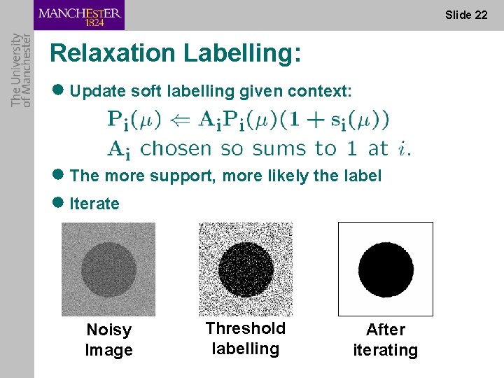
Slide 22 Relaxation Labelling: ● Update soft labelling given context: ● The more support, more likely the label ● Iterate Noisy Image Threshold labelling After iterating

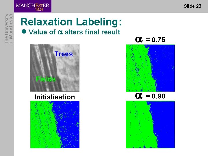
Slide 23 Relaxation Labeling: ● Value of alters final result = 0. 75 Trees Fields Initialisation = 0. 90

Segmentation as Optimisation

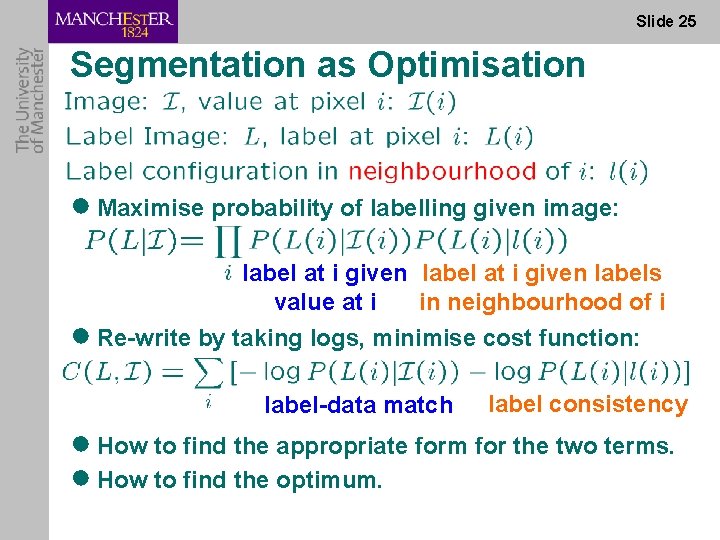
Slide 25 Segmentation as Optimisation ● Maximise probability of labelling given image: label at i given labels value at i in neighbourhood of i ● Re-write by taking logs, minimise cost function: label-data match label consistency ● How to find the appropriate form for the two terms. ● How to find the optimum.

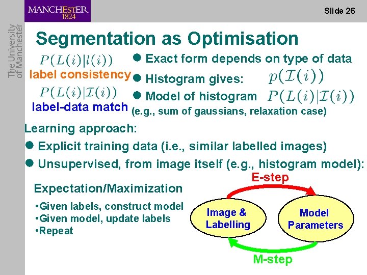
Slide 26 Segmentation as Optimisation ● Exact form depends on type of data label consistency ● Histogram gives: ● Model of histogram label-data match (e. g. , sum of gaussians, relaxation case) Learning approach: ● Explicit training data (i. e. , similar labelled images) ● Unsupervised, from image itself (e. g. , histogram model): E-step Expectation/Maximization • Given labels, construct model • Given model, update labels • Repeat Image & Labelling Model Parameters M-step

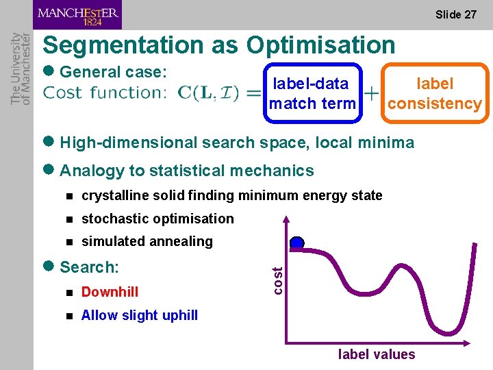
Slide 27 Segmentation as Optimisation ● General case: label-data match term label consistency ● High-dimensional search space, local minima ● Analogy to statistical mechanics crystalline solid finding minimum energy state n stochastic optimisation n simulated annealing ● Search: n Downhill n Allow slight uphill cost n label values

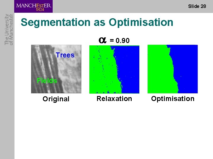
Slide 28 Segmentation as Optimisation = 0. 90 Trees Fields Original Relaxation Optimisation