Lecture 3 Monopoly Price discrimination Price discrimination and

Lecture 3, Monopoly Price discrimination

Price discrimination and monopoly • In the next section we look at price discrimination in the context of a single firm monopoly. • While this is useful in itself since there are many monopolies, the main purpose is in order to think about price discrimination in oligopolies; the lessons we learn in the monopoly case also hold true in a multi-firm case, but the analysis is simpler for a monopolist.

Price discrimination • Definition: An firm demonstrates price discrimination (PD) if it offers products to different consumers at different prices, and these differences are not solely due to cost differences. • Example 1: A movie theatre offers a student discount. The cost to theatre is the same regardless of customer, so this unambiguously qualifies as PD. • Example 2: A telephone company charges higher prices to rural consumers than to urban consumers. This is not PD if the price differential solely represents the higher average cost of providing phone services in low-density rural areas.

Further examples • Drug companies charge different prices in different countries? • Gas stations in different areas charge different prices? • Cellphone pricing plans? • Internet service? • Big Mac prices in different countries? • State universities, in-state tuition fees? • Weekend stay requirements for airline tickets?

Why price discriminate? • The advantage to firms of PD is that it can allow them to increase profits by capturing additional consumer surplus that they did not receive with a linear price. • From a welfare perspective, price discrimination is not necessarily undesirable. By implementing price discrimination, firms often charge a lower price to lowdemand consumers, and so sell to these consumers who would otherwise have not received the product at all. Thus, PD can mitigate the negative welfare effects of market power by increasing the quantity sold. • In the most extreme case (first degree price discrimination), welfare is the same as in perfect competition as producers capture all consumer surplus.

Requirements to price discriminate • In order for a firm to price discriminate successfully, several requirements must be met. • The firm must have some market power. • There must be different “types” of consumers with different marginal willingness to pay, and the firm must know this. • Arbitrage must be impossible (or very difficult). • Some forms of PD also have other requirements (in particular: the firm must be able to identify the type of a particular consumer).

Three forms of price discrimination • First degree price discrimination: personalized pricing. Every consumer offered a different price. • Second degree price discrimination: non-linear pricing. Firms offer menus of prices; consumers self-select into different groups. • Third degree price discrimination: linear pricing. Firms offer different linear prices to different consumer types.

Third-degree price discrimination • Under third-degree price discrimination, the firm offers a linear price for their product to different groups with different demands. • To implement this, consumer demand must differ by some observable characteristic, such as age, income, geographic location or education status. Different groups must have different willingness to pay. The firm must observe this willingness to pay, and can identify the type of a given consumer, and can prevent arbitrage between types. • The firm offers a price for each consumer type, and then each consumer can choose how much to buy at the price faced by their group.

3 rd degree PD examples • Adult, senior, student, child discounts. • Academic journals offering student, faculty, institutional/library prices. • Pharmaceutical prices in different countries. • Clip-out coupons. • Airline Sat night stay requirements. • Textbooks in US vs UK.

Implementing 3 rd deg PD • The strategy in 3 rd degree PD is fairly straightforward; the firm wishes to charge higher prices to types with more inelastic demand. • Typically we think about a “high type” consumer with high willingness to pay and a “low type” consumer with low willingness to pay; the equilibrium price to the high type will be higher than for the low type.

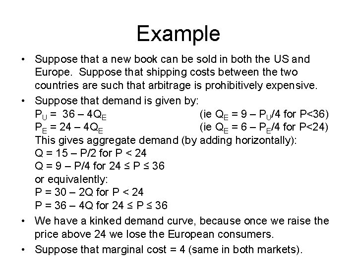
Example • Suppose that a new book can be sold in both the US and Europe. Suppose that shipping costs between the two countries are such that arbitrage is prohibitively expensive. • Suppose that demand is given by: PU = 36 – 4 QE (ie QE = 9 – PU/4 for P<36) PE = 24 – 4 QE (ie QE = 6 – PE/4 for P<24) This gives aggregate demand (by adding horizontally): Q = 15 – P/2 for P < 24 Q = 9 – P/4 for 24 ≤ P ≤ 36 or equivalently: P = 30 – 2 Q for P < 24 P = 36 – 4 Q for 24 ≤ P ≤ 36 • We have a kinked demand curve, because once we raise the price above 24 we lose the European consumers. • Suppose that marginal cost = 4 (same in both markets).

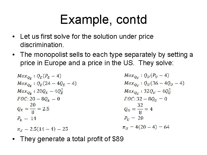
Example, contd • Let us first solve for the solution under price discrimination. • The monopolist sells to each type separately by setting a price in Europe and a price in the US. They solve: • They generate a total profit of $89

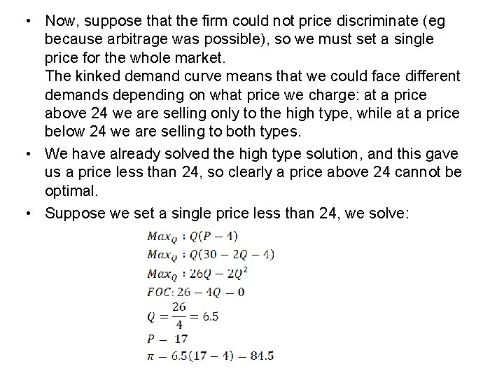
• Now, suppose that the firm could not price discriminate (eg because arbitrage was possible), so we must set a single price for the whole market. The kinked demand curve means that we could face different demands depending on what price we charge: at a price above 24 we are selling only to the high type, while at a price below 24 we are selling to both types. • We have already solved the high type solution, and this gave us a price less than 24, so clearly a price above 24 cannot be optimal. • Suppose we set a single price less than 24, we solve:

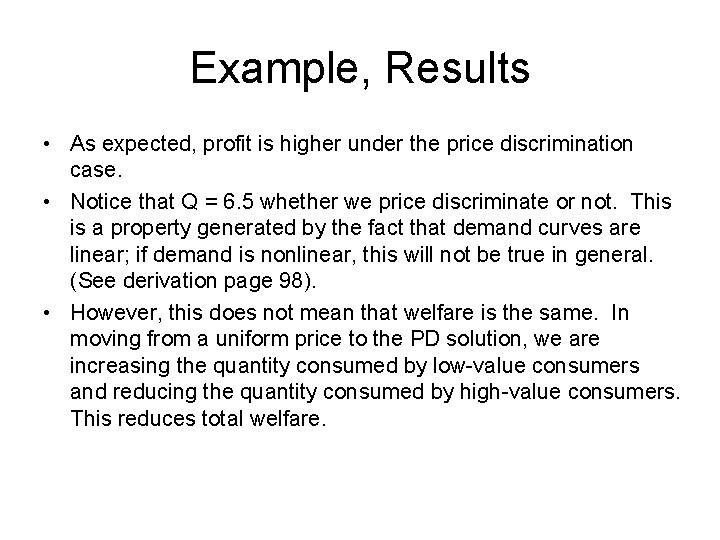
Example, Results • As expected, profit is higher under the price discrimination case. • Notice that Q = 6. 5 whether we price discriminate or not. This is a property generated by the fact that demand curves are linear; if demand is nonlinear, this will not be true in general. (See derivation page 98). • However, this does not mean that welfare is the same. In moving from a uniform price to the PD solution, we are increasing the quantity consumed by low-value consumers and reducing the quantity consumed by high-value consumers. This reduces total welfare.

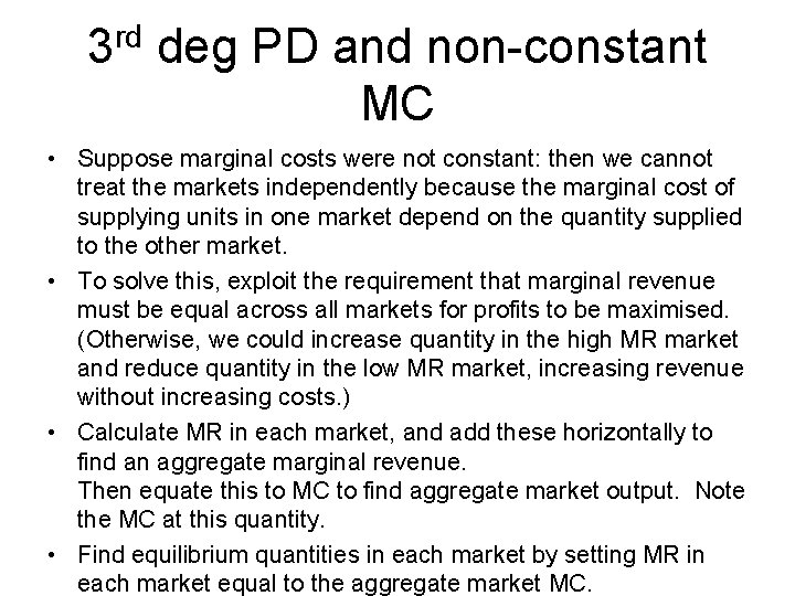
rd 3 deg PD and non-constant MC • Suppose marginal costs were not constant: then we cannot treat the markets independently because the marginal cost of supplying units in one market depend on the quantity supplied to the other market. • To solve this, exploit the requirement that marginal revenue must be equal across all markets for profits to be maximised. (Otherwise, we could increase quantity in the high MR market and reduce quantity in the low MR market, increasing revenue without increasing costs. ) • Calculate MR in each market, and add these horizontally to find an aggregate marginal revenue. Then equate this to MC to find aggregate market output. Note the MC at this quantity. • Find equilibrium quantities in each market by setting MR in each market equal to the aggregate market MC.

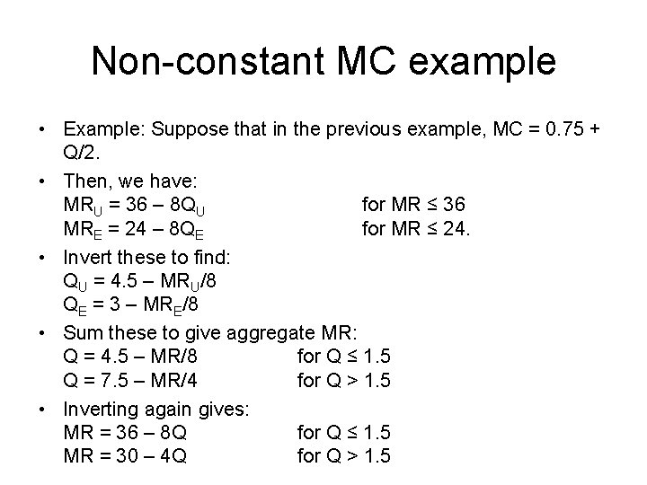
Non-constant MC example • Example: Suppose that in the previous example, MC = 0. 75 + Q/2. • Then, we have: MRU = 36 – 8 QU for MR ≤ 36 MRE = 24 – 8 QE for MR ≤ 24. • Invert these to find: QU = 4. 5 – MRU/8 QE = 3 – MRE/8 • Sum these to give aggregate MR: Q = 4. 5 – MR/8 for Q ≤ 1. 5 Q = 7. 5 – MR/4 for Q > 1. 5 • Inverting again gives: MR = 36 – 8 Q for Q ≤ 1. 5 MR = 30 – 4 Q for Q > 1. 5

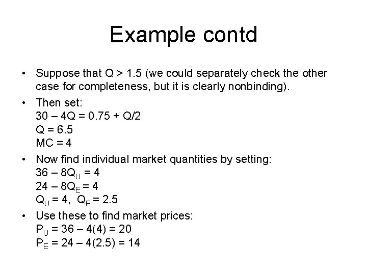
Example contd • Suppose that Q > 1. 5 (we could separately check the other case for completeness, but it is clearly nonbinding). • Then set: 30 – 4 Q = 0. 75 + Q/2 Q = 6. 5 MC = 4 • Now find individual market quantities by setting: 36 – 8 QU = 4 24 – 8 QE = 4 QU = 4, QE = 2. 5 • Use these to find market prices: PU = 36 – 4(4) = 20 PE = 24 – 4(2. 5) = 14

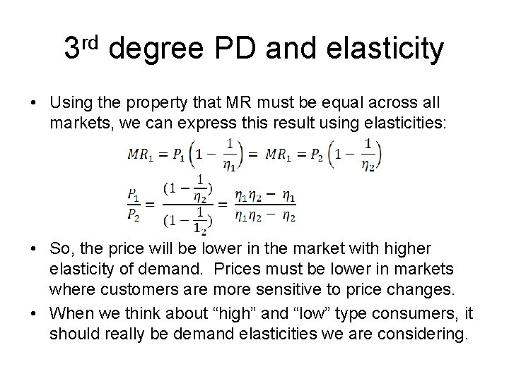
3 rd degree PD and elasticity • Using the property that MR must be equal across all markets, we can express this result using elasticities: • So, the price will be lower in the market with higher elasticity of demand. Prices must be lower in markets where customers are more sensitive to price changes. • When we think about “high” and “low” type consumers, it should really be demand elasticities we are considering.

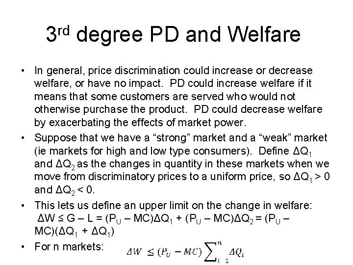
3 rd degree PD and Welfare • In general, price discrimination could increase or decrease welfare, or have no impact. PD could increase welfare if it means that some customers are served who would not otherwise purchase the product. PD could decrease welfare by exacerbating the effects of market power. • Suppose that we have a “strong” market and a “weak” market (ie markets for high and low type consumers). Define ΔQ 1 and ΔQ 2 as the changes in quantity in these markets when we move from discriminatory prices to a uniform price, so ΔQ 1 > 0 and ΔQ 2 < 0. • This lets us define an upper limit on the change in welfare: ΔW ≤ G – L = (PU – MC)ΔQ 1 + (PU – MC)ΔQ 2 = (PU – MC)(ΔQ 1 + ΔQ 1) • For n markets:

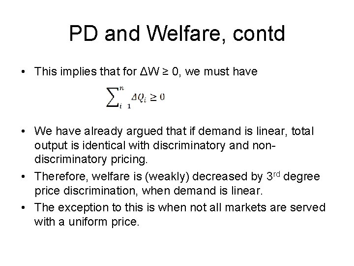
PD and Welfare, contd • This implies that for ΔW ≥ 0, we must have • We have already argued that if demand is linear, total output is identical with discriminatory and nondiscriminatory pricing. • Therefore, welfare is (weakly) decreased by 3 rd degree price discrimination, when demand is linear. • The exception to this is when not all markets are served with a uniform price.

PD and market exclusion • Suppose that demand for patented AIDS treatment is PN = 100 - QN in North America, and PN = α 100 - QN in Sub-Saharan Africa, with α < 1. • Suppose that marginal cost is constant, c = 20. • Suppose that the patentholder does not or cannot price discriminate across markets. Invert the demand functions QN = 100 – P, QS = α 100 – P. If the price is low enough to attract buyers in both markets then aggregate demand is Q = (1 + α)100 – 2 P, or equivalently P = (1 + α)50 – Q/2, and marginal revenue MR = (1 + α)(50 -Q). Imposing MC = MR gives Q = 30 + 50α, and P = 35 +25α. • Now recall our assumption that both markets are served without price discrimination: then it must hold that the equilibrium price is less than the maximum price (=100α) that African consumers are willing to pay. That is, it must be that 35 +25α < 100α, which is true only if α > 35/75 = 0. 4666.