Lecture 3 Improving Neural Network Training part 2

Lecture 3: Improving Neural Network Training (part 2, preliminary version) Reading and Research in Deep Learning James K Baker

Programming Assignment Due Feb 27 • Program feedforward, backprop, and stochastic gradient descent with minibatches in Cython. Do multiple random • Choose at least one of the tutorial data sets initializations and/or multiple cross • Experiment with at least three of the following • • • Sigmoid vs Re. LU Cost functions If your problem requires CNN Number of nodes or RNN/LSTM, choose from Number of layers the additional relevant Learning rate hyperparameters. Regularization parameter Size of minibatch Momentum Adagrad, Ada. Delta, RMSprop, ADAM • Prepare slides showing the results of your experiments • Report your difficulties, bugs, time for each subtask • Do not post your code. Send it privately to me validations. Compare. Report the change in program running time as key routines are implemented in C. The best and most interesting will be selected for presentation in class. Learn from your mistakes. Post interim reports by noon each Wednesday. Final report due Feb 27. Post on Piazza or other site set up by Infra team.

Major Project Alternative • Choose a paper that reports a record in a competitive benchmark within the last 3 years • Implementing the techniques in the paper, or your own improvements, compare your results to those in the paper and any more recent results • Differences from more research-oriented major project: • Competitive challenge • Not necessary to read and gist collection of other research papers • Should be comparable amount of work • Difference with unrestricted competitive challenge • If you are restricted because of computing resources or other problem, you can still get a good grade if you do well on a scaleddown version of the problem (as with the other research paper major projects)

Challenge Projects (possible follow-ons to course) • Two challenges: • 1) Develop a CMU framework (ala Theano, Caffe, Torch) • 2) Develop an open competition testbed and set a benchmark result • Design a testbed that is accessible to students and individual researchers and hobbyists. • Should be feasible on a single computer with a high-end GPU board • However, the task should be hard enough for humans so that deep learning can demonstrate near-human performance or better

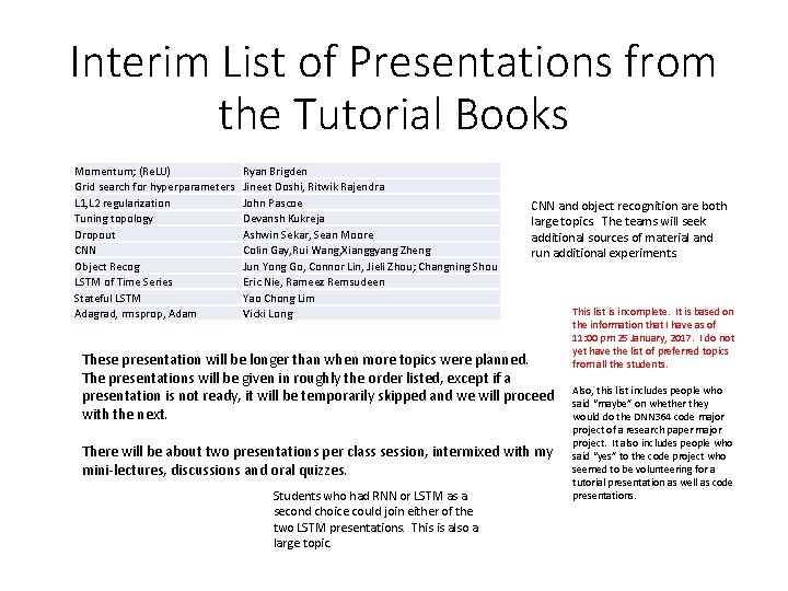
Interim List of Presentations from the Tutorial Books Momentum; (Re. LU) Grid search for hyperparameters L 1, L 2 regularization Tuning topology Dropout CNN Object Recog LSTM of Time Series Stateful LSTM Adagrad, rmsprop, Adam Ryan Brigden Jineet Doshi, Ritwik Rajendra John Pascoe Devansh Kukreja Ashwin Sekar, Sean Moore Colin Gay, Rui Wang, Xianggyang Zheng Jun Yong Go, Connor Lin, Jieli Zhou; Changning Shou Eric Nie, Rameez Remsudeen Yao Chong Lim Vicki Long CNN and object recognition are both large topics. The teams will seek additional sources of material and run additional experiments. These presentation will be longer than when more topics were planned. The presentations will be given in roughly the order listed, except if a presentation is not ready, it will be temporarily skipped and we will proceed with the next. There will be about two presentations per class session, intermixed with my mini-lectures, discussions and oral quizzes. Students who had RNN or LSTM as a second choice could join either of the two LSTM presentations. This is also a large topic. This list is incomplete. It is based on the information that I have as of 11: 00 pm 25 January, 2017. I do not yet have the list of preferred topics from all the students. Also, this list includes people who said “maybe” on whether they would do the DNN 364 code major project of a research paper major project. It also includes people who said “yes” to the code project who seemed to be volunteering for a tutorial presentation as well as code presentations.

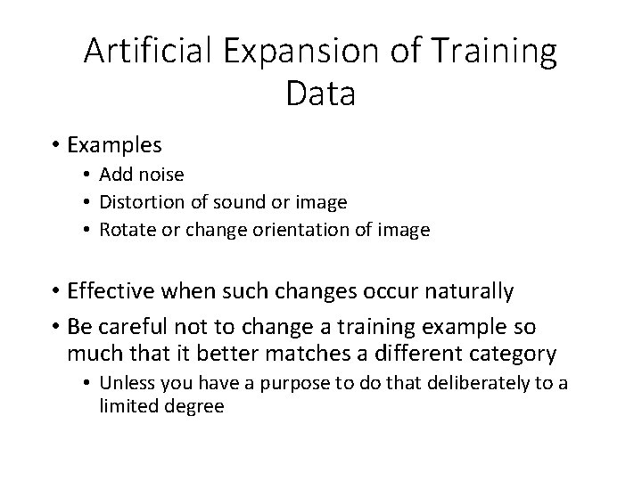
Artificial Expansion of Training Data • Examples • Add noise • Distortion of sound or image • Rotate or change orientation of image • Effective when such changes occur naturally • Be careful not to change a training example so much that it better matches a different category • Unless you have a purpose to do that deliberately to a limited degree

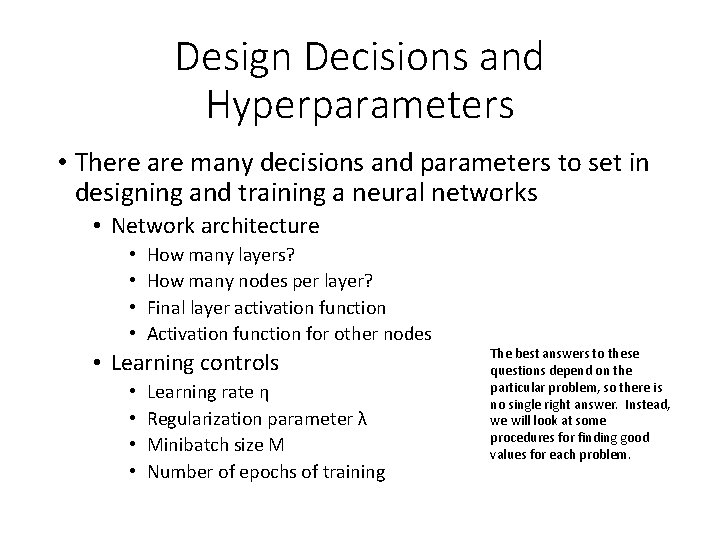
Design Decisions and Hyperparameters • There are many decisions and parameters to set in designing and training a neural networks • Network architecture • • How many layers? How many nodes per layer? Final layer activation function Activation function for other nodes • Learning controls • • Learning rate η Regularization parameter λ Minibatch size M Number of epochs of training The best answers to these questions depend on the particular problem, so there is no single right answer. Instead, we will look at some procedures for finding good values for each problem.

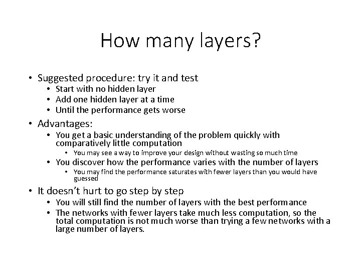
How many layers? • Suggested procedure: try it and test • Start with no hidden layer • Add one hidden layer at a time • Until the performance gets worse • Advantages: • You get a basic understanding of the problem quickly with comparatively little computation • You may see a way to improve your design without wasting so much time • You discover how the performance varies with the number of layers • You may find the performance saturates with fewer layers than you would have guessed • It doesn’t hurt to go step by step • You will still find the number of layers with the best performance • The networks with fewer layers take much less computation, so the total computation is not much worse than trying a few networks with a large number of layers.

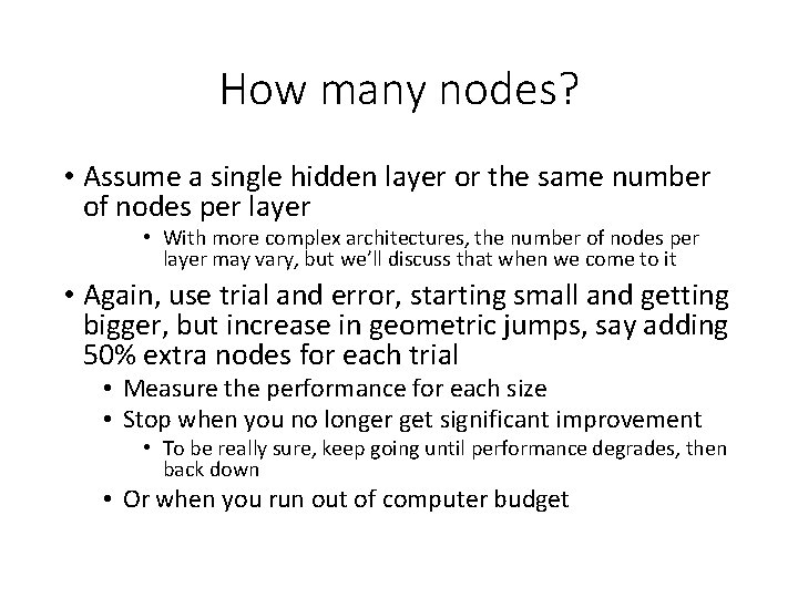
How many nodes? • Assume a single hidden layer or the same number of nodes per layer • With more complex architectures, the number of nodes per layer may vary, but we’ll discuss that when we come to it • Again, use trial and error, starting small and getting bigger, but increase in geometric jumps, say adding 50% extra nodes for each trial • Measure the performance for each size • Stop when you no longer get significant improvement • To be really sure, keep going until performance degrades, then back down • Or when you run out of computer budget

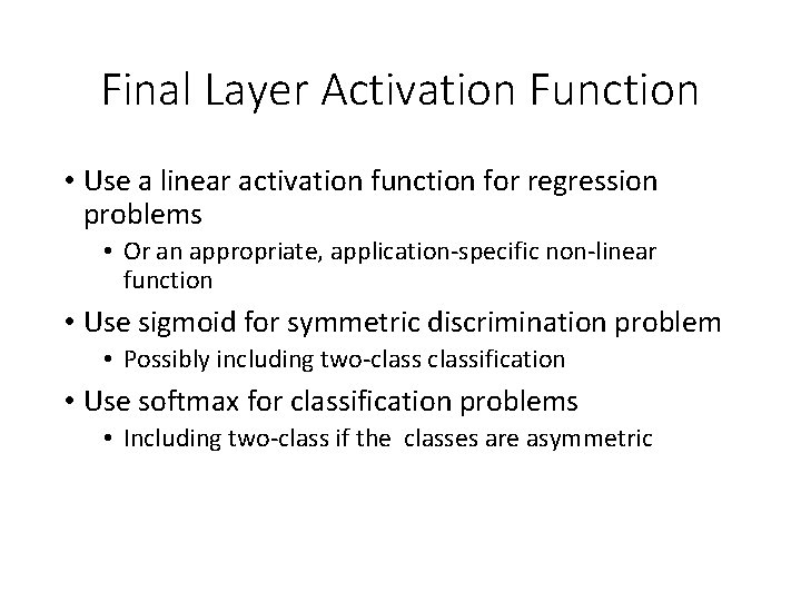
Final Layer Activation Function • Use a linear activation function for regression problems • Or an appropriate, application-specific non-linear function • Use sigmoid for symmetric discrimination problem • Possibly including two-classification • Use softmax for classification problems • Including two-class if the classes are asymmetric

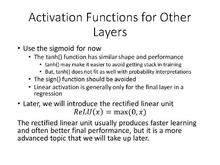
Activation Functions for Other Layers •

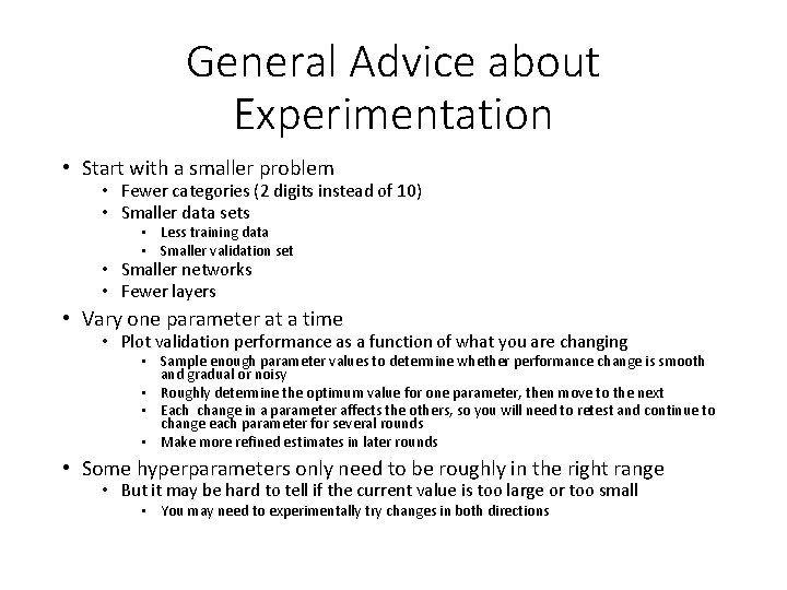
General Advice about Experimentation • Start with a smaller problem • Fewer categories (2 digits instead of 10) • Smaller data sets • Less training data • Smaller validation set • Smaller networks • Fewer layers • Vary one parameter at a time • Plot validation performance as a function of what you are changing • Sample enough parameter values to determine whether performance change is smooth and gradual or noisy • Roughly determine the optimum value for one parameter, then move to the next • Each change in a parameter affects the others, so you will need to retest and continue to change each parameter for several rounds • Make more refined estimates in later rounds • Some hyperparameters only need to be roughly in the right range • But it may be hard to tell if the current value is too large or too small • You may need to experimentally try changes in both directions

The Learning Rate η • When the learning rate is set too high, the performance on the validation set will fluctuate • When the learning rate is too low, the performance will improve smoothly, but learning will be slow • The optimum performance would be at the highest learning rate that doesn’t produce fluctuations (called the threshold value), but that performance would be disturbed by changes in other parameters • Suggestion: Find the threshold value by trial and error, then back off, say, by a factor of 2.

The Learning Rate η (cont. ) • Note: Nielsen suggests evaluating the performance of η on the training data rather than the validation data as with the other parameters • This makes sense, although it might not matter much • The learning rate is optimized not for performance, but to speed up the rate of convergence in training • The training is guaranteed to converge on the training data (in the limit of an infinite amount of data) but is not guaranteed to converge on the validation data • However, either method will usually give similar results.

Stopping Early • You don’t need to set the number of epochs of training as a fixed parameter • If the gradient were known exactly, you could make sure that every step would be an improvement by making the learning step arbitrarily small • This would guarantee convergence • However, we only have a statistical estimate of the gradient, so the performance will fluctuate even with a low learning rate • Train until fluctuations begin, then train somewhat more to see if progress will resume • After continuing for a reasonable time without further improvement, stop!

The Regularization Parameter λ • The regularization parameter forces the learning toward a smoother function • This is ideal if the observed data is generated by a smooth function with added noise • But, we don’t know the true function or how smooth it might be • If λ is too large, it will smooth the model more than the true function • If λ is too small, it will not smooth out as much of the noise

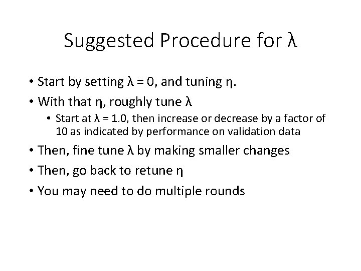
Suggested Procedure for λ • Start by setting λ = 0, and tuning η. • With that η, roughly tune λ • Start at λ = 1. 0, then increase or decrease by a factor of 10 as indicated by performance on validation data • Then, fine tune λ by making smaller changes • Then, go back to retune η • You may need to do multiple rounds

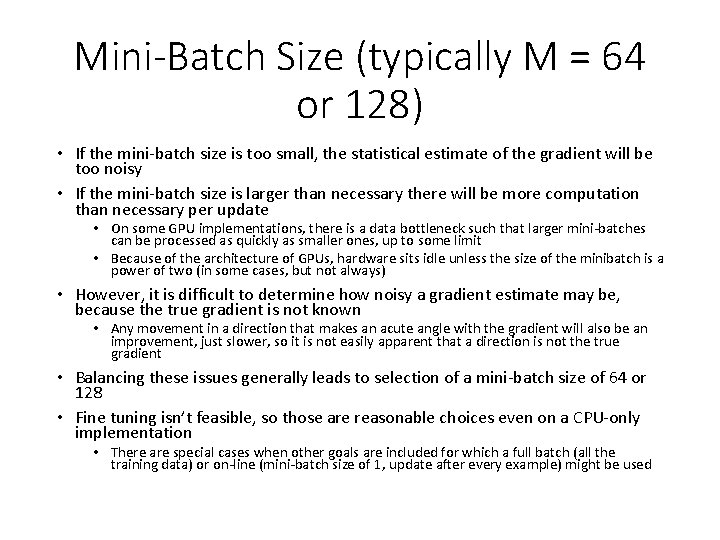
Mini-Batch Size (typically M = 64 or 128) • If the mini-batch size is too small, the statistical estimate of the gradient will be too noisy • If the mini-batch size is larger than necessary there will be more computation than necessary per update • On some GPU implementations, there is a data bottleneck such that larger mini-batches can be processed as quickly as smaller ones, up to some limit • Because of the architecture of GPUs, hardware sits idle unless the size of the minibatch is a power of two (in some cases, but not always) • However, it is difficult to determine how noisy a gradient estimate may be, because the true gradient is not known • Any movement in a direction that makes an acute angle with the gradient will also be an improvement, just slower, so it is not easily apparent that a direction is not the true gradient • Balancing these issues generally leads to selection of a mini-batch size of 64 or 128 • Fine tuning isn’t feasible, so those are reasonable choices even on a CPU-only implementation • There are special cases when other goals are included for which a full batch (all the training data) or on-line (mini-batch size of 1, update after every example) might be used

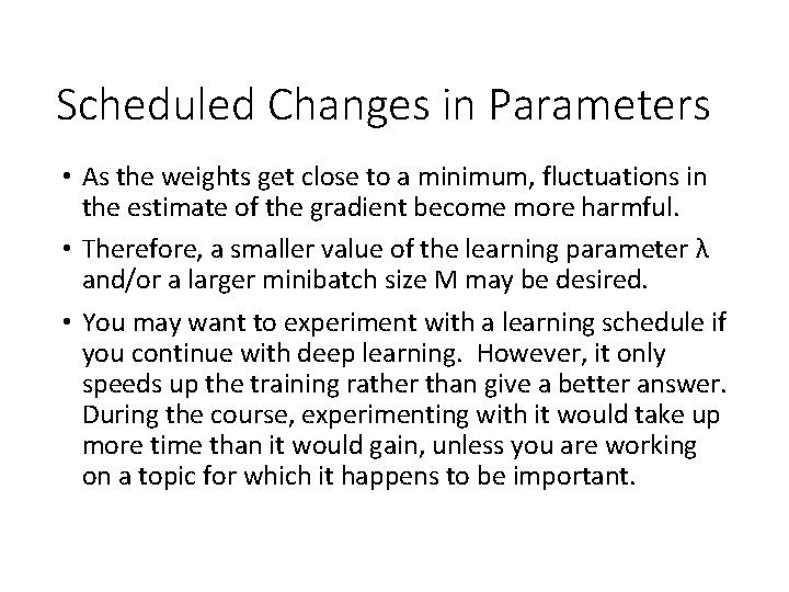
Scheduled Changes in Parameters • As the weights get close to a minimum, fluctuations in the estimate of the gradient become more harmful. • Therefore, a smaller value of the learning parameter λ and/or a larger minibatch size M may be desired. • You may want to experiment with a learning schedule if you continue with deep learning. However, it only speeds up the training rather than give a better answer. During the course, experimenting with it would take up more time than it would gain, unless you are working on a topic for which it happens to be important.

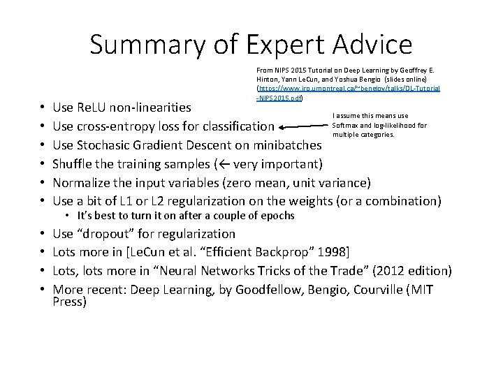
Summary of Expert Advice From NIPS 2015 Tutorial on Deep Learning by Geoffrey E. Hinton, Yann Le. Cun, and Yoshua Bengio (slides online) (https: //www. iro. umontreal. ca/~bengioy/talks/DL-Tutorial -NIPS 2015. pdf) • • • Use Re. LU non-linearities I assume this means use Softmax and log-likelihood for Use cross-entropy loss for classification multiple categories. Use Stochasic Gradient Descent on minibatches Shuffle the training samples (← very important) Normalize the input variables (zero mean, unit variance) Use a bit of L 1 or L 2 regularization on the weights (or a combination) • • Use “dropout” for regularization Lots more in [Le. Cun et al. “Efficient Backprop” 1998] Lots, lots more in “Neural Networks Tricks of the Trade” (2012 edition) More recent: Deep Learning, by Goodfellow, Bengio, Courville (MIT Press) • It’s best to turn it on after a couple of epochs

Other learning improvement techniques • Rectified linear units (Re. LU) • Momentum • Nesterov’s method • Rmsprop • Adagrad • Adam • Other network topologies and techniques • CNN, BPTT, RNN, LSTM

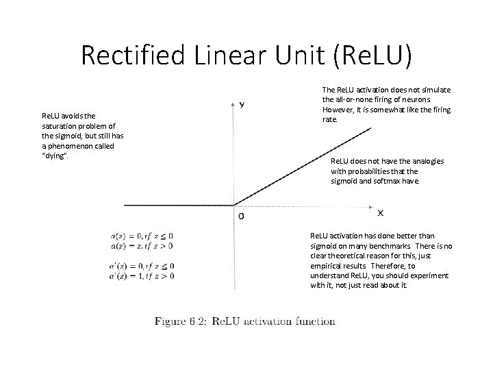
Rectified Linear Unit (Re. LU) Re. LU avoids the saturation problem of the sigmoid, but still has a phenomenon called “dying”. The Re. LU activation does not simulate the all-or-none firing of neurons. However, it is somewhat like the firing rate. Re. LU does not have the analogies with probabilities that the sigmoid and softmax have. Re. LU activation has done better than sigmoid on many benchmarks. There is no clear theoretical reason for this, just empirical results. Therefore, to understand Re. LU, you should experiment with it, not just read about it.

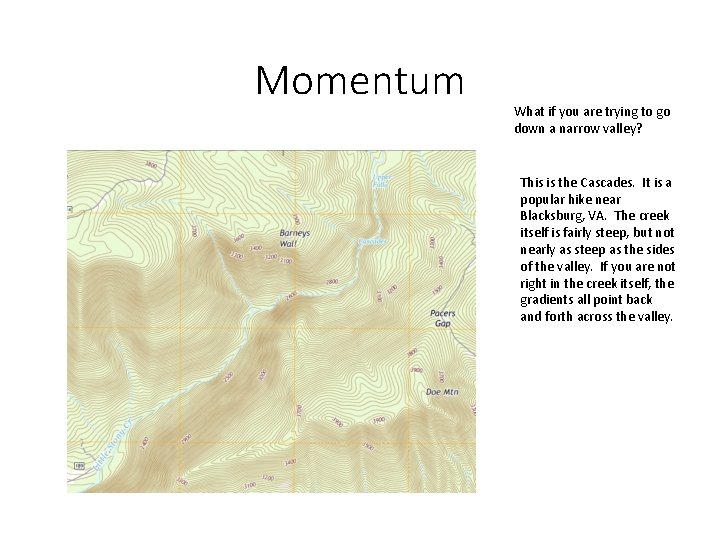
Momentum What if you are trying to go down a narrow valley? This is the Cascades. It is a popular hike near Blacksburg, VA. The creek itself is fairly steep, but not nearly as steep as the sides of the valley. If you are not right in the creek itself, the gradients all point back and forth across the valley.

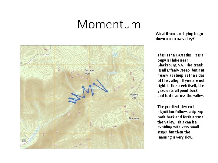
Momentum What if you are trying to go down a narrow valley? This is the Cascades. It is a popular hike near Blacksburg, VA. The creek itself is fairly steep, but not nearly as steep as the sides of the valley. If you are not right in the creek itself, the gradients all point back and forth across the valley. The gradient descent algorithm follows a zig-zag path back and forth across the valley. This can be avoiding with very small steps, but then the learning is very slow.

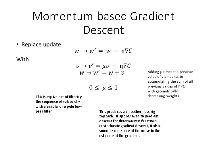
Momentum-based Gradient Descent • This is equivalent of filtering the sequence of values of v with a simple, one-pole lowpass filter. This produces a smoother, less zigzag path. It applies even to gradient descent for deterministic functions. In stochastic gradient descent, it also smooths out some of the noise in the estimate of the gradient.

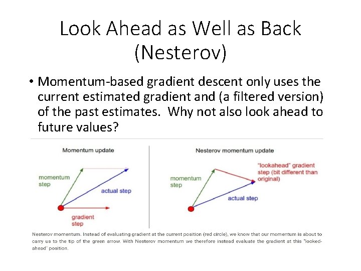
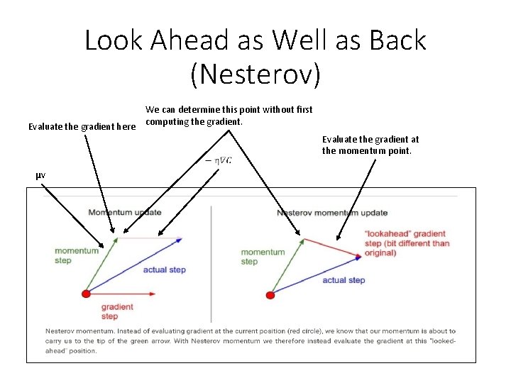
Look Ahead as Well as Back (Nesterov) • Momentum-based gradient descent only uses the current estimated gradient and (a filtered version) of the past estimates. Why not also look ahead to future values?

Look Ahead as Well as Back (Nesterov) Evaluate the gradient here We can determine this point without first computing the gradient. Evaluate the gradient at the momentum point. μv

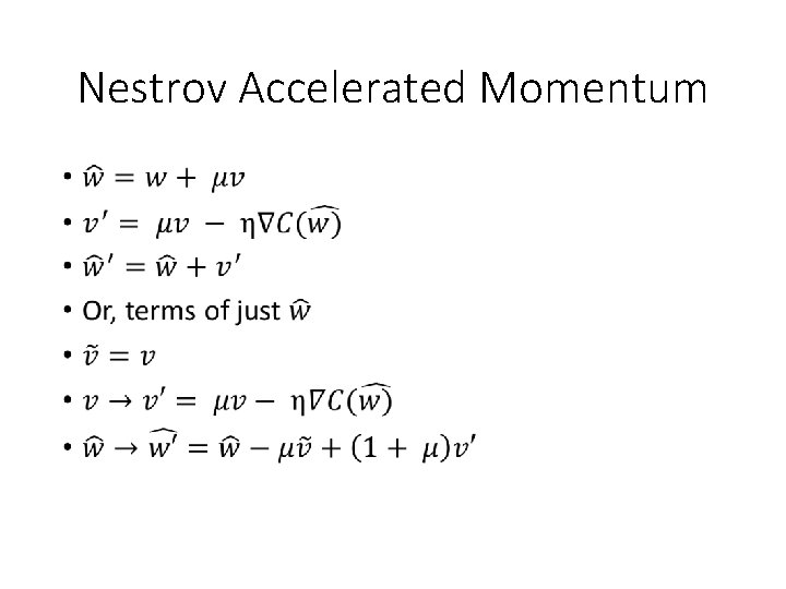
Nestrov Accelerated Momentum •

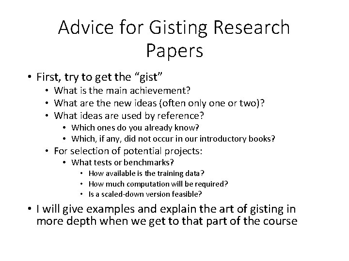
Advice for Gisting Research Papers • First, try to get the “gist” • What is the main achievement? • What are the new ideas (often only one or two)? • What ideas are used by reference? • Which ones do you already know? • Which, if any, did not occur in our introductory books? • For selection of potential projects: • What tests or benchmarks? • How available is the training data? • How much computation will be required? • Is a scaled-down version feasible? • I will give examples and explain the art of gisting in more depth when we get to that part of the course

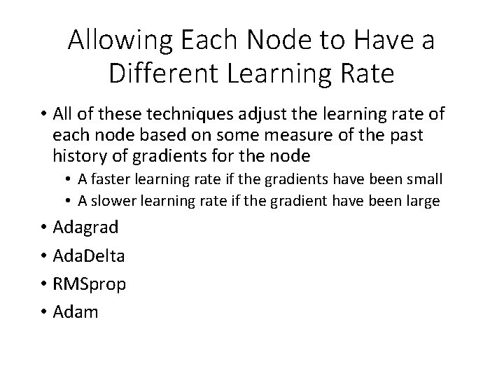
Allowing Each Node to Have a Different Learning Rate • All of these techniques adjust the learning rate of each node based on some measure of the past history of gradients for the node • A faster learning rate if the gradients have been small • A slower learning rate if the gradient have been large • Adagrad • Ada. Delta • RMSprop • Adam

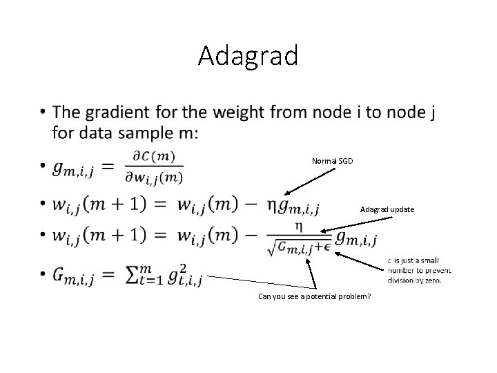
Adagrad • Normal SGD Adagrad update Can you see a potential problem?

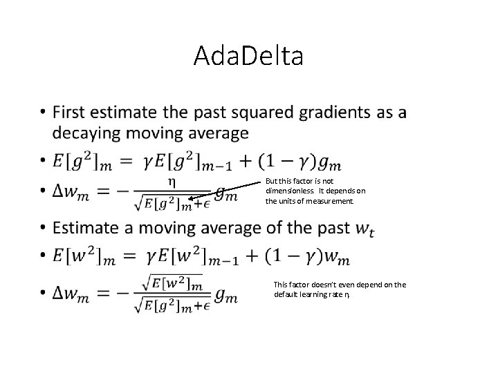
Ada. Delta • But this factor is not dimensionless. It depends on the units of measurement. This factor doesn’t even depend on the default learning rate η.

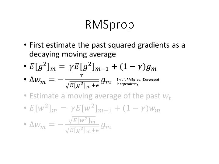
RMSprop • This is RMSprop. Developed independently.

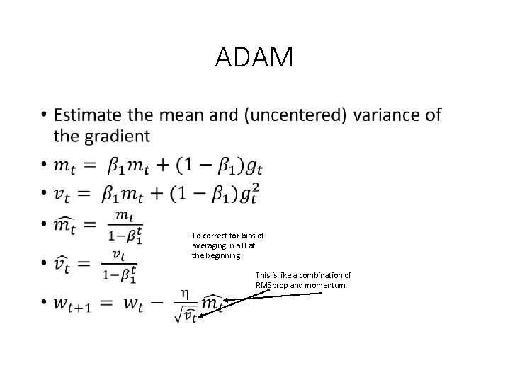
ADAM • To correct for bias of averaging in a 0 at the beginning. This is like a combination of RMSprop and momentum.

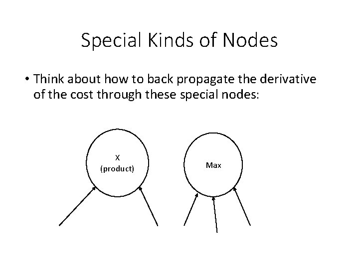
Special Kinds of Nodes • Think about how to back propagate the derivative of the cost through these special nodes: X (product) Max

More to Come … • Additional topics will be covered as mini-lectures • Ignore the rest of the slides (if any), they are not yet finished.