Lecture 3 Images and convolutional neural networks Practical

Lecture 3: Images and convolutional neural networks Practical deep learning 1

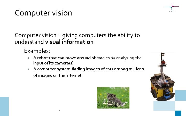
Computer vision = giving computers the ability to understand visual information Examples: ○ A robot that can move around obstacles by analysing the input of its camera(s) ○ A computer system finding images of cats among millions of images on the Internet 2

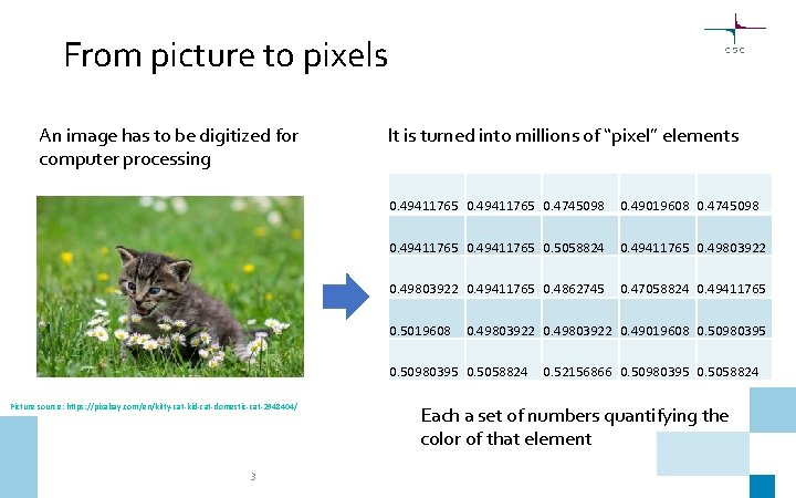
From picture to pixels An image has to be digitized for computer processing It is turned into millions of “pixel” elements 0. 49411765 0. 4745098 0. 49019608 0. 4745098 0. 49411765 0. 5058824 0. 49411765 0. 49803922 0. 49411765 0. 4862745 0. 47058824 0. 49411765 0. 5019608 0. 49803922 0. 49019608 0. 50980395 0. 5058824 Picture source: https: //pixabay. com/en/kitty-cat-kid-cat-domestic-cat-2948404/ 3 0. 52156866 0. 50980395 0. 5058824 Each a set of numbers quantifying the color of that element

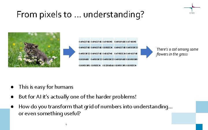
From pixels to … understanding? 0. 49411765 0. 4745098 0. 49019608 0. 4745098 0. 49411765 0. 5058824 0. 49411765 0. 49803922 0. 49411765 0. 4862745 0. 47058824 0. 49411765 There’s a cat among some flowers in the grass 0. 5019608 0. 49803922 0. 49019608 0. 50980395 0. 5058824 0. 52156866 0. 50980395 0. 5058824 ● This is easy for humans ● But for AI it’s actually one of the harder problems! ● How do you transform that grid of numbers into understanding… or even something useful? 4

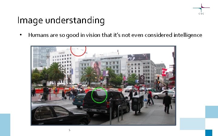
Image understanding • Humans are so good in vision that it’s not even considered intelligence 5

Convolutional neural networks

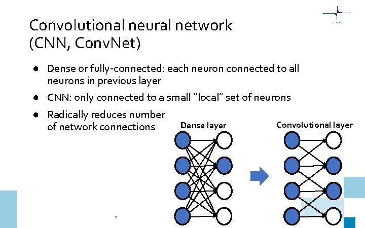
Convolutional neural network (CNN, Conv. Net) ● Dense or fully-connected: each neuron connected to all neurons in previous layer ● CNN: only connected to a small “local” set of neurons ● Radically reduces number of network connections 7 Dense layer Convolutional layer

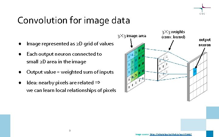
Convolution for image data 3✕ 3 image area 3✕ 3 weights (conv. kernel) ● Image represented as 2 D grid of values ● Each output neuron connected to small 2 D area in the image ● Output value = weighted sum of inputs ● Idea: nearby pixels are related ⇒ we can learn local relationships of pixels 8 Image source: https: //mlnotebook. github. io/post/CNN 1/ output neuron

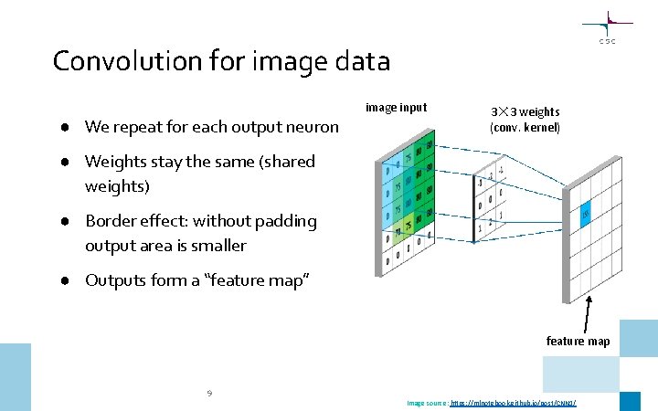
Convolution for image data ● We repeat for each output neuron image input 3✕ 3 weights (conv. kernel) ● Weights stay the same (shared weights) ● Border effect: without padding output area is smaller ● Outputs form a “feature map” feature map 9 Image source: https: //mlnotebook. github. io/post/CNN 1/

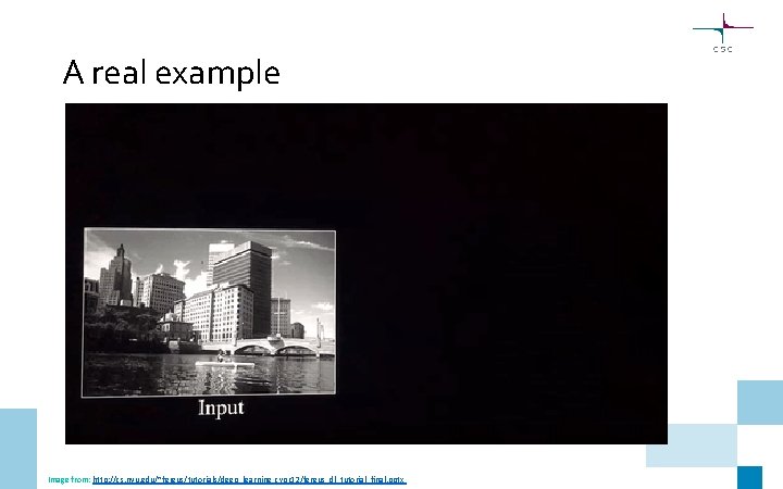
A real example Image from: http: //cs. nyu. edu/~fergus/tutorials/deep_learning_cvpr 12/fergus_dl_tutorial_final. pptx

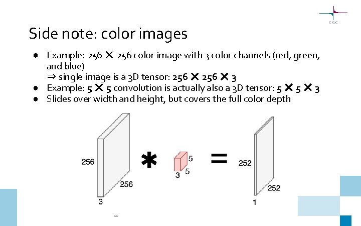
Side note: color images ● Example: 256 ✕ 256 color image with 3 color channels (red, green, and blue) ⇒ single image is a 3 D tensor: 256 ✕ 3 ● Example: 5 ✕ 5 convolution is actually also a 3 D tensor: 5 ✕ 3 ● Slides over width and height, but covers the full color depth 11

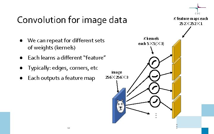
Convolution for image data K feature maps each 252✕ 1 K kernels each 5✕ 5(✕ 3) ● We can repeat for different sets of weights (kernels) ● Each learns a different “feature” ● Typically: edges, corners, etc ● Each outputs a feature map image 256✕ 3 . . . 12

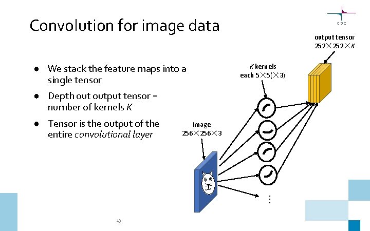
Convolution for image data ● We stack the feature maps into a single tensor output tensor 252✕K K kernels each 5✕ 5(✕ 3) ● Depth output tensor = number of kernels K ● Tensor is the output of the entire convolutional layer image 256✕ 3 . . . 13

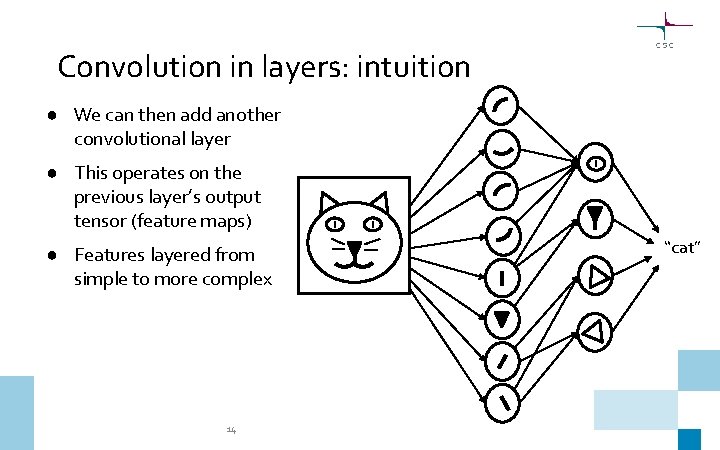
Convolution in layers: intuition ● We can then add another convolutional layer ● This operates on the previous layer’s output tensor (feature maps) ● Features layered from simple to more complex 14 “cat”

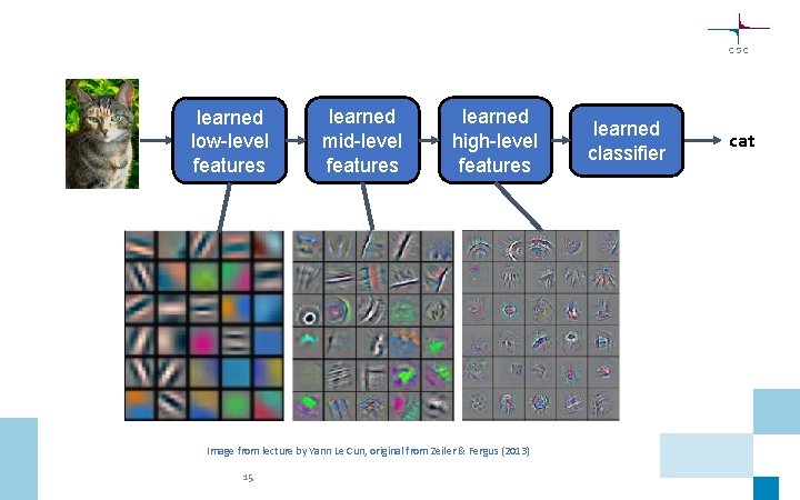
learned low-level features learned mid-level features learned high-level features Image from lecture by Yann Le Cun, original from Zeiler & Fergus (2013) 15 learned classifier cat

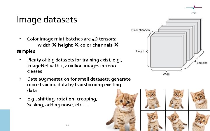
Image datasets Color image mini-batches are 4 D tensors: width ✕ height ✕ color channels ✕ samples • • Plenty of big datasets for training exist, e. g. , Image. Net with 1, 2 million images in 1000 classes Data augmentation for small datasets: generate more training data by transforming existing data E. g. , shifting, rotation, cropping, Scaling, adding noise, etc … 16

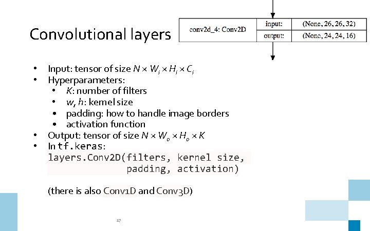
Convolutional layers • • Input: tensor of size N × Wi × Hi × Ci Hyperparameters: • K: number of filters • w, h: kernel size • padding: how to handle image borders • activation function Output: tensor of size N × Wo × Ho × K In tf. keras: layers. Conv 2 D(filters, kernel_size, padding, activation) (there is also Conv 1 D and Conv 3 D) 17

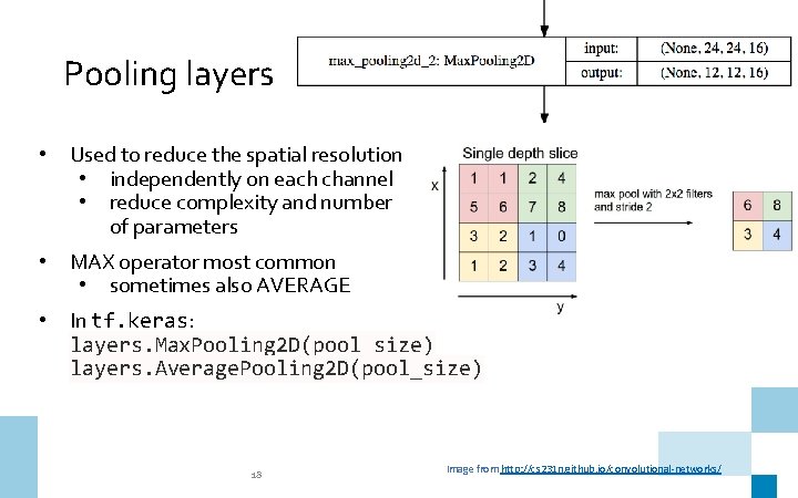
Pooling layers • Used to reduce the spatial resolution • independently on each channel • reduce complexity and number of parameters • MAX operator most common • sometimes also AVERAGE • In tf. keras: layers. Max. Pooling 2 D(pool_size) layers. Average. Pooling 2 D(pool_size) 18 Image from http: //cs 231 n. github. io/convolutional-networks/

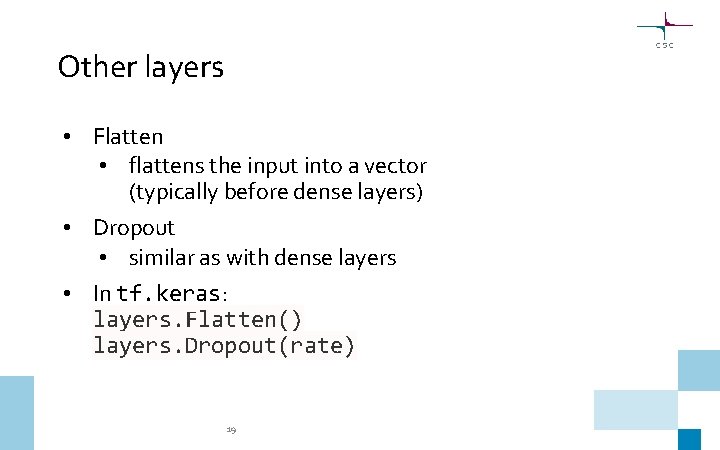
Other layers • Flatten • flattens the input into a vector (typically before dense layers) • Dropout • similar as with dense layers • In tf. keras: layers. Flatten() layers. Dropout(rate) 19

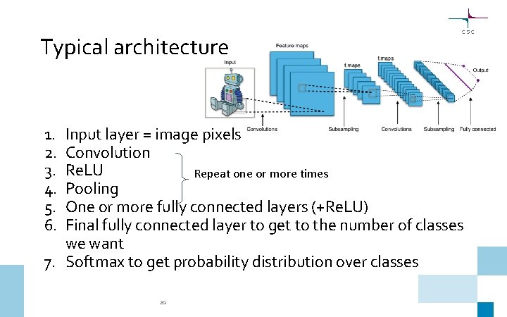
Typical architecture 1. 2. 3. 4. 5. 6. Input layer = image pixels Convolution Re. LU Repeat one or more times Pooling One or more fully connected layers (+Re. LU) Final fully connected layer to get to the number of classes we want 7. Softmax to get probability distribution over classes 20

CNN architectures and applications 21

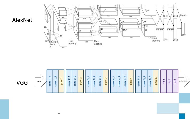
Alex. Net VGG 22

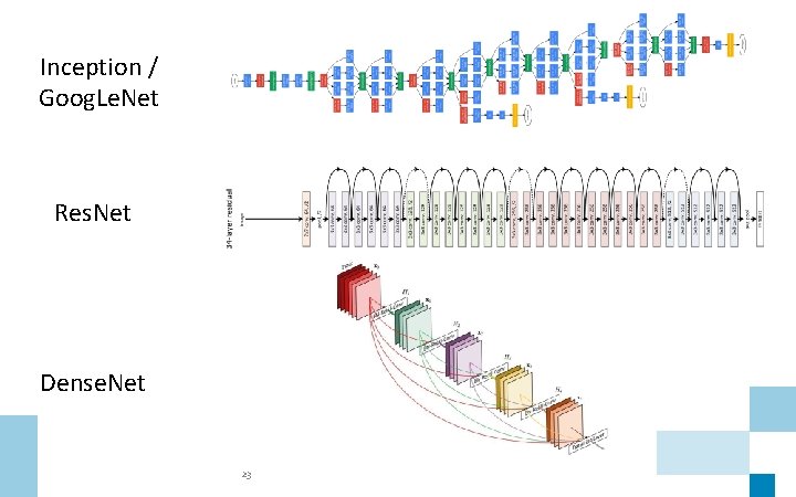
Inception / Goog. Le. Net Res. Net Dense. Net 23

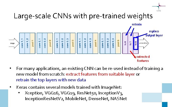
Large-scale CNNs with pre-trained weights retrain replace output layer extracted features • For many applications, an existing CNN can be re-used instead of training a new model from scratch: extract features from suitable layer or retrain the top layers with new data • Keras contains several models trained with Image. Net: • Xception, VGG 16, VGG 19, Res. Net 50, Inception. V 3, Inception. Res. Net. V 2, Mobile. Net, Dense. Net, NASNet

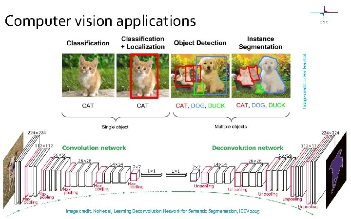
Image credit: Li Fei-Fei et al Computer vision applications 25 Image credit: Noh et al, Learning Deconvolution Network for Semantic Segmentation, ICCV 2015

Some selected applications • Object detection: https: //pjreddie. com/darknet/yolo/ • Semantic segmentation: https: //www. youtube. com/watch? v=q. Wl 9 ids. Cu. LQ • Human pose estimation: https: //www. youtube. com/watch? v=p. W 6 n. ZXe. Wl. GM • Video recognition: https: //valossa. com/ • Digital pathology: https: //www. aiforia. com/ 26