Lecture 3 Finding Edges CSE 6367 Computer Vision

Lecture 3 Finding Edges CSE 6367 – Computer Vision Spring 2010 Vassilis Athitsos University of Texas at Arlington

Vertical and Horizontal Edges • Consider the image as a function f(i, j) mapping pixels to intensity values. – Function f(i, j) can be seen as a discretized version of a more general function g(y, x), mapping pairs of real numbers to intensity values. – Vertical edges correspond to points in g with high dg/dx. – Horizontal edges correspond to points in g with high dg/dy.

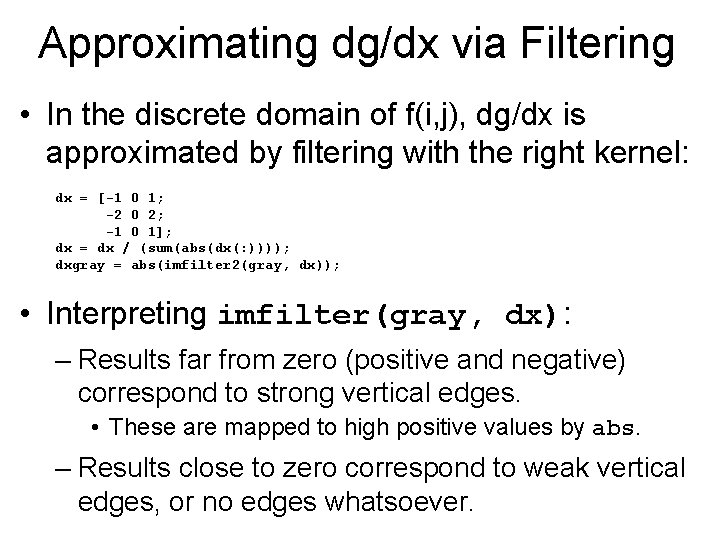
Approximating dg/dx via Filtering • In the discrete domain of f(i, j), dg/dx is approximated by filtering with the right kernel: dx = [-1 0 1; -2 0 2; -1 0 1]; dx = dx / (sum(abs(dx(: )))); dxgray = abs(imfilter 2(gray, dx)); • Interpreting imfilter(gray, dx): – Results far from zero (positive and negative) correspond to strong vertical edges. • These are mapped to high positive values by abs. – Results close to zero correspond to weak vertical edges, or no edges whatsoever.

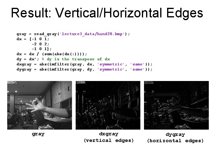
Result: Vertical/Horizontal Edges gray = read_gray('lecture 3_data/hand 20. bmp'); dx = [-1 0 1; -2 0 2; -1 0 1]; dx = dx / (sum(abs(dx(: )))); dy = dx’; % dy is the transpose of dx dxgray = abs(imfilter(gray, dx, 'symmetric', 'same')); dygray = abs(imfilter(gray, dy, 'symmetric', 'same')); gray dxgray (vertical edges) dygray (horizontal edges)

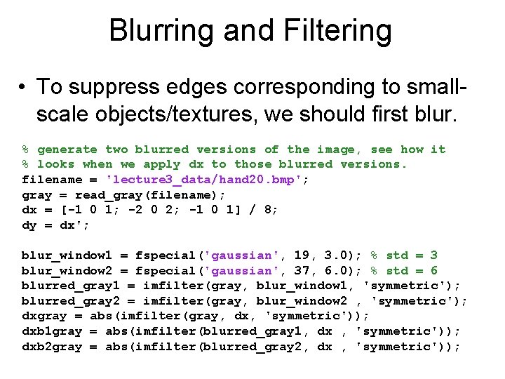
Blurring and Filtering • To suppress edges corresponding to smallscale objects/textures, we should first blur. % generate two blurred versions of the image, see how it % looks when we apply dx to those blurred versions. filename = 'lecture 3_data/hand 20. bmp'; gray = read_gray(filename); dx = [-1 0 1; -2 0 2; -1 0 1] / 8; dy = dx'; blur_window 1 = fspecial('gaussian', 19, 3. 0); % std = 3 blur_window 2 = fspecial('gaussian', 37, 6. 0); % std = 6 blurred_gray 1 = imfilter(gray, blur_window 1, 'symmetric'); blurred_gray 2 = imfilter(gray, blur_window 2 , 'symmetric'); dxgray = abs(imfilter(gray, dx, 'symmetric')); dxb 1 gray = abs(imfilter(blurred_gray 1, dx , 'symmetric')); dxb 2 gray = abs(imfilter(blurred_gray 2, dx , 'symmetric'));

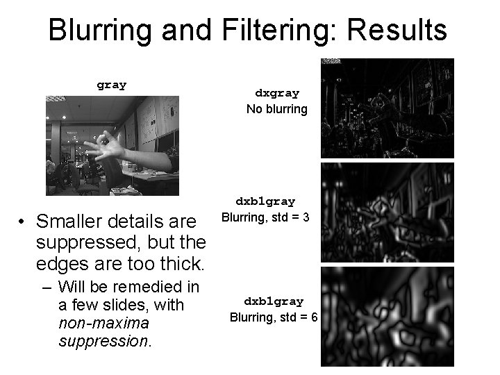
Blurring and Filtering: Results gray • Smaller details are suppressed, but the edges are too thick. – Will be remedied in a few slides, with non-maxima suppression. dxgray No blurring dxb 1 gray Blurring, std = 3 dxb 1 gray Blurring, std = 6

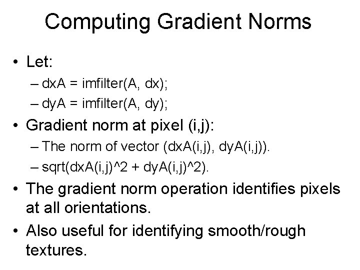
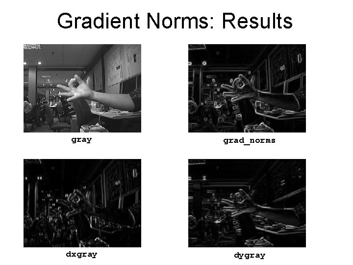
Computing Gradient Norms • Let: – dx. A = imfilter(A, dx); – dy. A = imfilter(A, dy); • Gradient norm at pixel (i, j): – The norm of vector (dx. A(i, j), dy. A(i, j)). – sqrt(dx. A(i, j)^2 + dy. A(i, j)^2). • The gradient norm operation identifies pixels at all orientations. • Also useful for identifying smooth/rough textures.

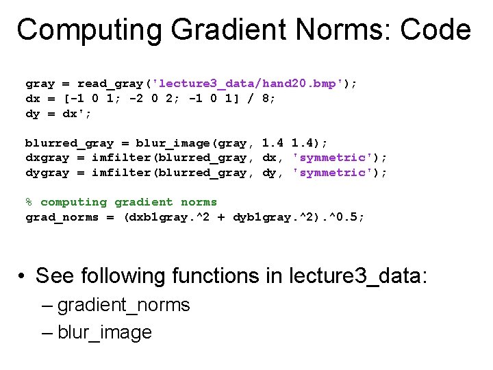
Computing Gradient Norms: Code gray = read_gray('lecture 3_data/hand 20. bmp'); dx = [-1 0 1; -2 0 2; -1 0 1] / 8; dy = dx'; blurred_gray = blur_image(gray, 1. 4); dxgray = imfilter(blurred_gray, dx, 'symmetric'); dygray = imfilter(blurred_gray, dy, 'symmetric'); % computing gradient norms grad_norms = (dxb 1 gray. ^2 + dyb 1 gray. ^2). ^0. 5; • See following functions in lecture 3_data: – gradient_norms – blur_image

Gradient Norms: Results gray grad_norms dxgray dygray

Notes on Gradient Norms • Gradient norms detect edges at all orientations. • However, gradient norms in themselves are not a good output for an edge detector: – We need thinner edges. – We need to decide which pixels are edge pixels.