Lecture 3 Decision Theory Chapter 5 S 1

Lecture 3 Decision Theory Chapter 5 S 1

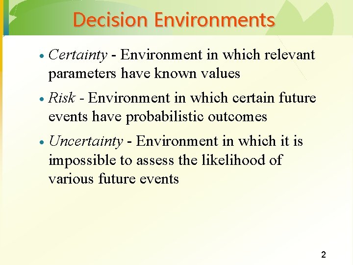
Decision Environments · Certainty - Environment in which relevant parameters have known values · Risk - Environment in which certain future events have probabilistic outcomes · Uncertainty - Environment in which it is impossible to assess the likelihood of various future events 2

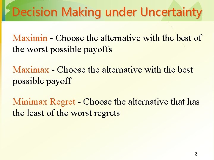
Decision Making under Uncertainty Maximin - Choose the alternative with the best of the worst possible payoffs Maximax - Choose the alternative with the best possible payoff Minimax Regret - Choose the alternative that has the least of the worst regrets 3

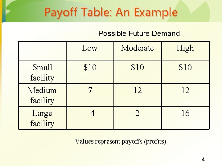
Payoff Table: An Example Possible Future Demand Small facility Medium facility Large facility Low Moderate High $10 $10 7 12 12 -4 2 16 Values represent payoffs (profits) 4

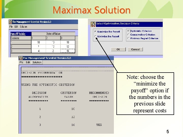
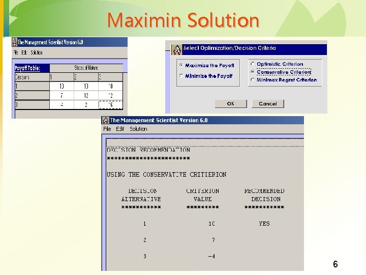
Maximax Solution Note: choose the “minimize the payoff” option if the numbers in the previous slide represent costs 5

Maximin Solution 6

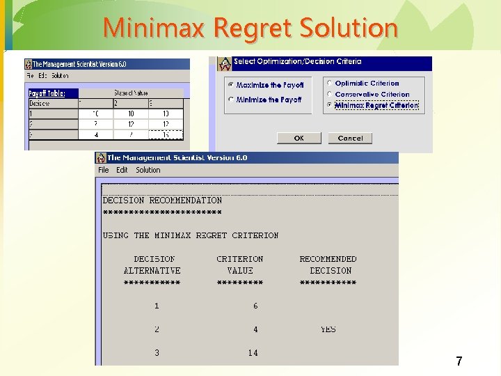
Minimax Regret Solution 7

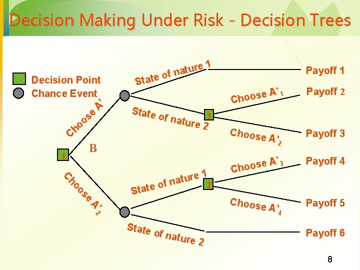
Decision Making Under Risk - Decision Trees Decision Point Chance Event ’ A e s o o h C State ture a n f o of nat 1 ho C 1 e r u t f na 2 o e t a e os St ’ 2 A State of nat ure 2 A’ 1 e s o o Ch Payoff 2 Choose A’ 2 Payoff 3 e. A s o o h C ’ 3 Payoff 4 Choose A’ 4 Payoff 5 2 ure 2 B 1 Payoff 6 8

Decision Making with Probabilities · Expected Value Approach Useful if probabilistic information regarding the states of nature is available · Expected return for each decision is calculated by summing the products of the payoff under each state of nature and the probability of the respective state of nature occurring · Decision yielding the best expected return is chosen. · 9

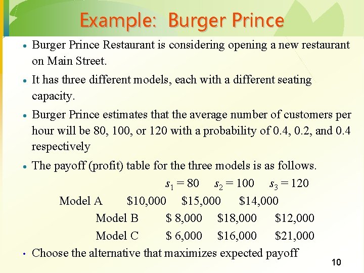
Example: Burger Prince · Burger Prince Restaurant is considering opening a new restaurant on Main Street. · It has three different models, each with a different seating capacity. · Burger Prince estimates that the average number of customers per hour will be 80, 100, or 120 with a probability of 0. 4, 0. 2, and 0. 4 respectively · The payoff (profit) table for the three models is as follows. s 1 = 80 s 2 = 100 s 3 = 120 Model A $10, 000 $15, 000 $14, 000 Model B $ 8, 000 $12, 000 Model C $ 6, 000 $16, 000 $21, 000 Choose the alternative that maximizes expected payoff • 10

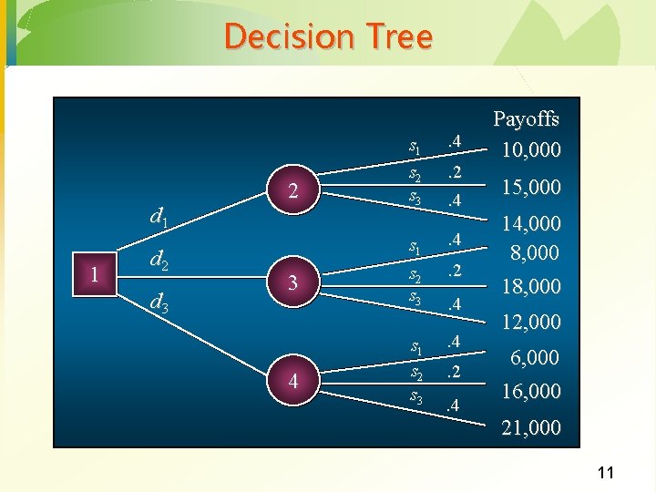
Decision Tree d 1 1 d 2 d 3 2 3 4 s 1 s 2 s 3 . 4. 2. 4 Payoffs 10, 000 15, 000 14, 000 8, 000 12, 000 6, 000 16, 000 21, 000 11

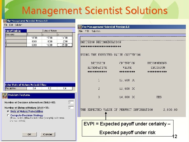
Management Scientist Solutions EVPI = Expected payoff under certainty – Expected payoff under risk 12

Lecture 2 Forecasting Chapter 3 13

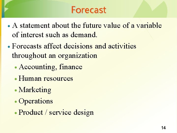
Forecast A statement about the future value of a variable of interest such as demand. · Forecasts affect decisions and activities throughout an organization · Accounting, finance · Human resources · Marketing · Operations · Product / service design · 14

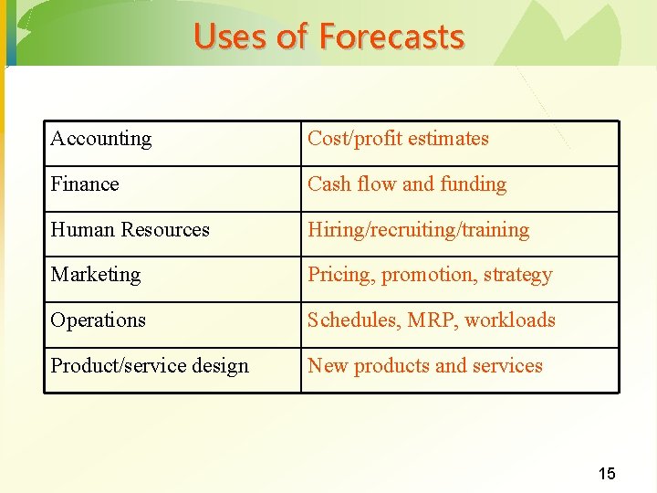
Uses of Forecasts Accounting Cost/profit estimates Finance Cash flow and funding Human Resources Hiring/recruiting/training Marketing Pricing, promotion, strategy Operations Schedules, MRP, workloads Product/service design New products and services 15

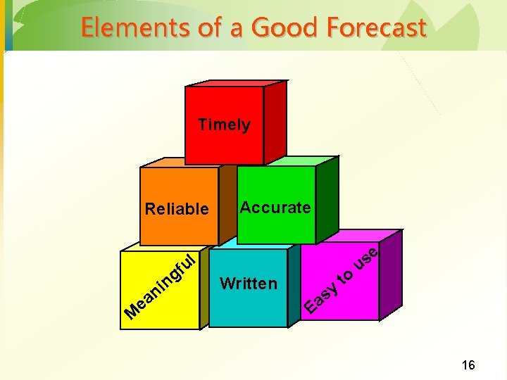
Elements of a Good Forecast Timely Reliable ul M e f g n i an Accurate Written y s Ea to e s u 16

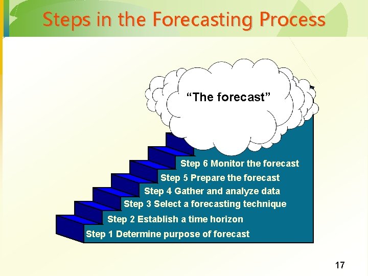
Steps in the Forecasting Process “The forecast” Step 6 Monitor the forecast Step 5 Prepare the forecast Step 4 Gather and analyze data Step 3 Select a forecasting technique Step 2 Establish a time horizon Step 1 Determine purpose of forecast 17

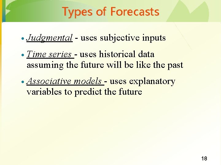
Types of Forecasts · Judgmental - uses subjective inputs · Time series - uses historical data assuming the future will be like the past · Associative models - uses explanatory variables to predict the future 18

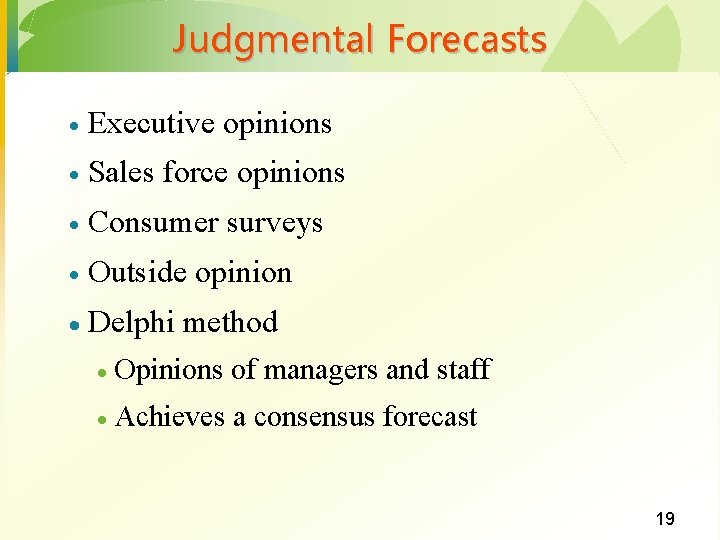
Judgmental Forecasts · Executive opinions · Sales force opinions · Consumer surveys · Outside opinion · Delphi method · Opinions of managers and staff · Achieves a consensus forecast 19

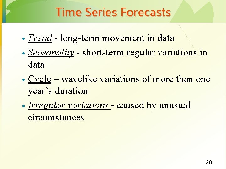
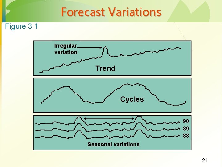
Time Series Forecasts Trend - long-term movement in data · Seasonality - short-term regular variations in data · Cycle – wavelike variations of more than one year’s duration · Irregular variations - caused by unusual circumstances · 20

Forecast Variations Figure 3. 1 Irregular variation Trend Cycles 90 89 88 Seasonal variations 21

Smoothing/Averaging Methods Used in cases in which the time series is fairly stable and has no significant trend, seasonal, or cyclical effects · Purpose of averaging - to smooth out the irregular components of the time series. · Four common smoothing/averaging methods are: · Moving averages · Weighted moving averages · Exponential smoothing · 22

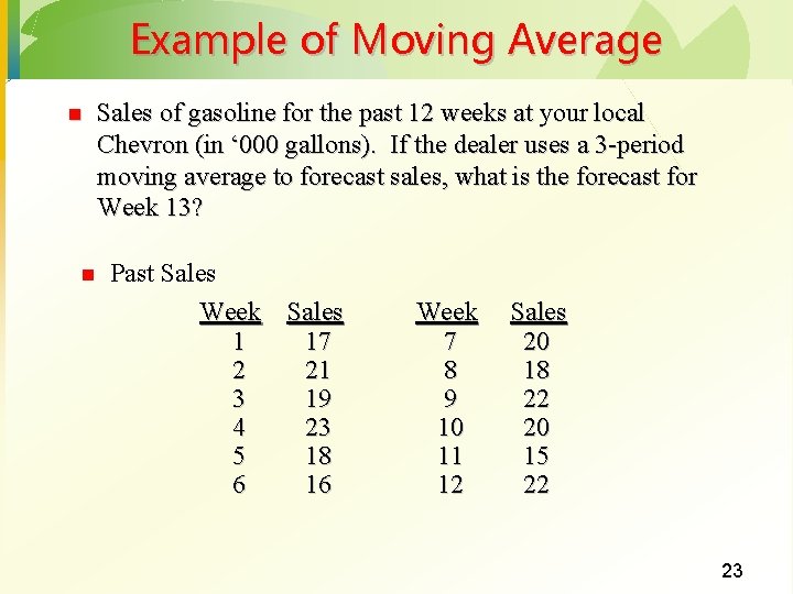
Example of Moving Average n n Sales of gasoline for the past 12 weeks at your local Chevron (in ‘ 000 gallons). If the dealer uses a 3 -period moving average to forecast sales, what is the forecast for Week 13? Past Sales Week Sales 1 17 2 21 3 19 4 23 5 18 6 16 Week 7 8 9 10 11 12 Sales 20 18 22 20 15 22 23

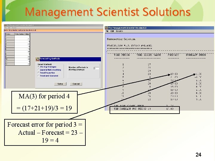
Management Scientist Solutions MA(3) for period 4 = (17+21+19)/3 = 19 Forecast error for period 3 = Actual – Forecast = 23 – 19 = 4 24

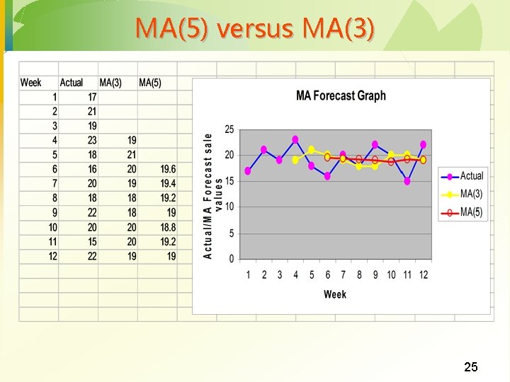
MA(5) versus MA(3) 25

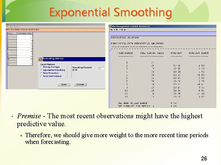
Exponential Smoothing • Premise - The most recent observations might have the highest predictive value. · Therefore, we should give more weight to the more recent time periods when forecasting. 26

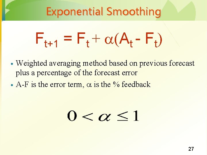
Exponential Smoothing Ft+1 = Ft + (At - Ft) · · Weighted averaging method based on previous forecast plus a percentage of the forecast error A-F is the error term, is the % feedback 27

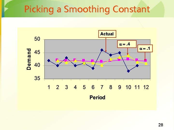
Picking a Smoothing Constant Actual . 4 . 1 28

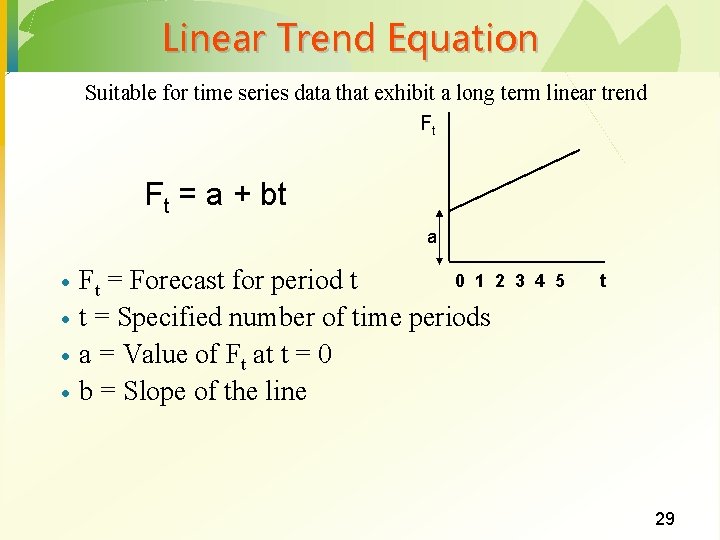
Linear Trend Equation Suitable for time series data that exhibit a long term linear trend Ft Ft = a + bt a · · 0 1 2 Ft = Forecast for period t t = Specified number of time periods a = Value of Ft at t = 0 b = Slope of the line 3 4 5 t 29

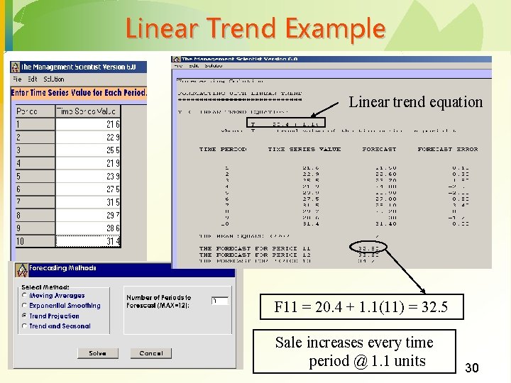
Linear Trend Example Linear trend equation F 11 = 20. 4 + 1. 1(11) = 32. 5 Sale increases every time period @ 1. 1 units 30

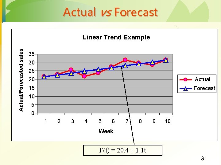
Actual vs Forecast Actual/Forecasted sales Linear Trend Example 35 30 25 20 Actual 15 Forecast 10 5 0 1 2 3 4 5 6 7 8 9 10 Week F(t) = 20. 4 + 1. 1 t 31

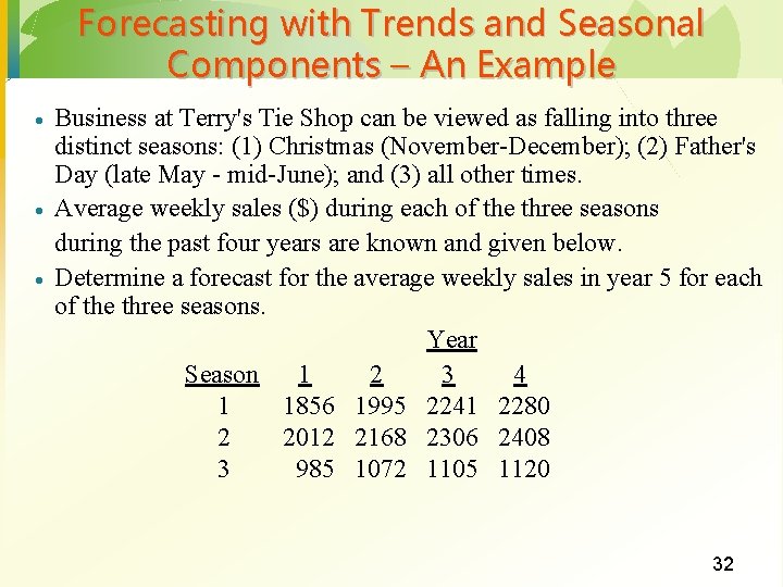
Forecasting with Trends and Seasonal Components – An Example · · · Business at Terry's Tie Shop can be viewed as falling into three distinct seasons: (1) Christmas (November-December); (2) Father's Day (late May - mid-June); and (3) all other times. Average weekly sales ($) during each of the three seasons during the past four years are known and given below. Determine a forecast for the average weekly sales in year 5 for each of the three seasons. Year Season 1 2 3 4 1 1856 1995 2241 2280 2 2012 2168 2306 2408 3 985 1072 1105 1120 32

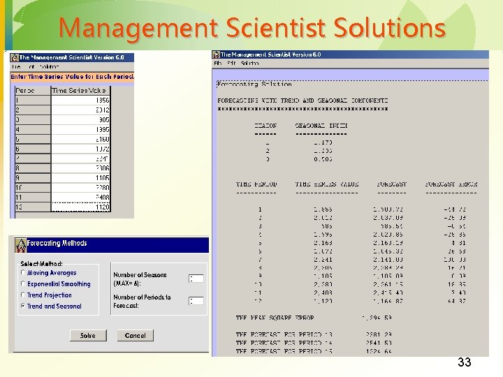
Management Scientist Solutions 33

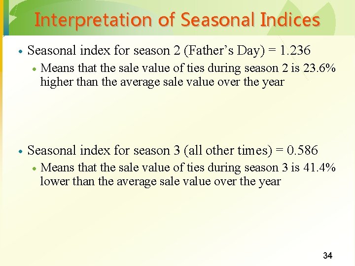
Interpretation of Seasonal Indices · Seasonal index for season 2 (Father’s Day) = 1. 236 · · Means that the sale value of ties during season 2 is 23. 6% higher than the average sale value over the year Seasonal index for season 3 (all other times) = 0. 586 · Means that the sale value of ties during season 3 is 41. 4% lower than the average sale value over the year 34

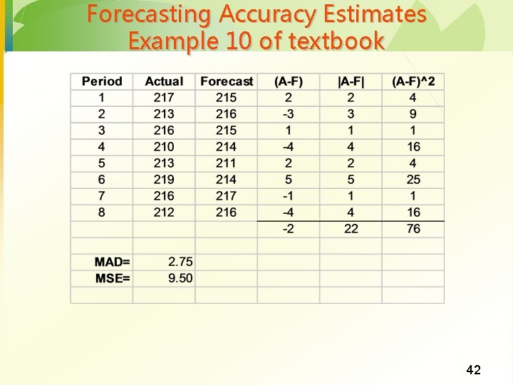
Forecast Accuracy · Error - difference between actual value and predicted value · Mean Absolute Deviation (MAD) · Average · absolute error Mean Squared Error (MSE) · Average of squared error 35

Associative Forecasting · Predictor variables - used to predict values of variable interest · Regression - technique for fitting a line to a set of points · Least squares line - minimizes sum of squared deviations around the line 36

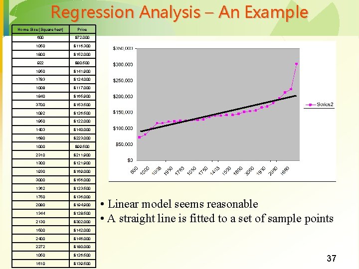
Regression Analysis – An Example Home-Size (Square feet) Price 600 $72, 000 1050 $116, 300 1800 $152, 000 922 $80, 500 1950 $141, 900 1783 $124, 000 1008 $117, 000 1840 $165, 900 3700 $153, 500 1092 $126, 500 1950 $122, 000 1403 $140, 000 1680 $223, 000 1000 $99, 500 2310 $211, 900 1300 $121, 900 1930 $169, 000 3000 $156, 000 1362 $123, 500 1750 $136, 000 2080 $194, 900 1344 $128, 500 2130 $302, 000 1500 $142, 000 2400 $146, 000 2272 $180, 000 1050 $126, 500 1610 $139, 500 • Linear model seems reasonable • A straight line is fitted to a set of sample points 37

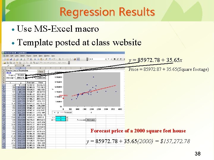
Regression Results Use MS-Excel macro · Template posted at class website · y = 85972. 78 + 35. 65 x Price = 85972. 87 + 35. 65(Square footage) Forecast price of a 2000 square feet house y = 85972. 78 + 35. 65(2000) = $157, 272. 78 38

Forecast Accuracy · Error - difference between actual value and predicted value · Mean Absolute Deviation (MAD) · Average · absolute error Mean Squared Error (MSE) · Average of squared error 39

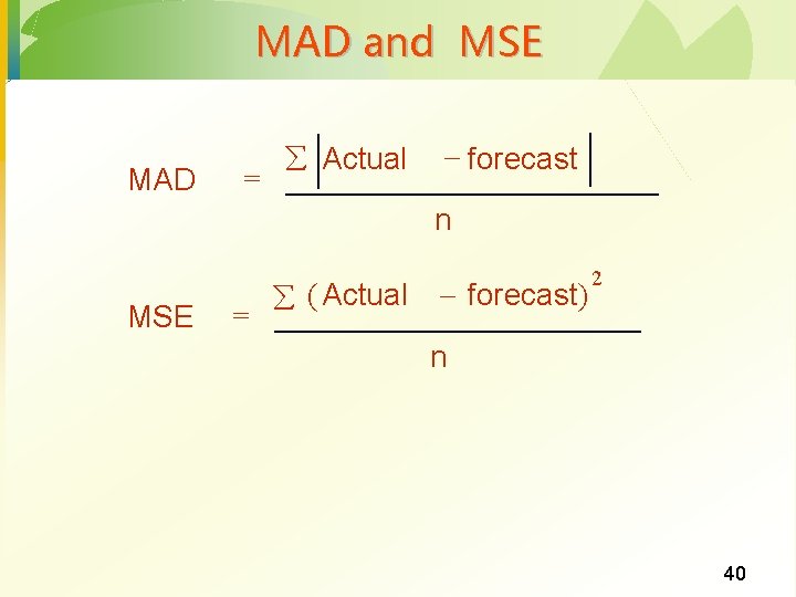
MAD and MSE MAD = Actual forecast n MSE = ( Actual forecast) 2 n 40

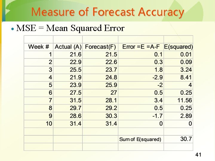
Measure of Forecast Accuracy · MSE = Mean Squared Error 41

Forecasting Accuracy Estimates Example 10 of textbook 42

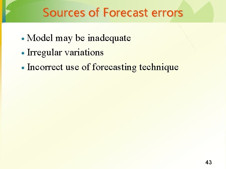
Sources of Forecast errors Model may be inadequate · Irregular variations · Incorrect use of forecasting technique · 43

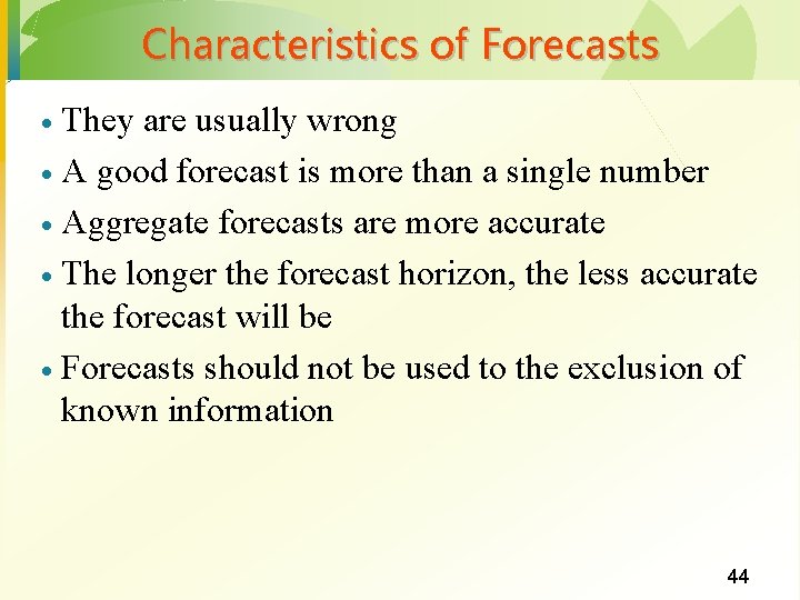
Characteristics of Forecasts They are usually wrong · A good forecast is more than a single number · Aggregate forecasts are more accurate · The longer the forecast horizon, the less accurate the forecast will be · Forecasts should not be used to the exclusion of known information · 44

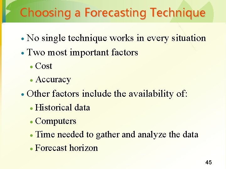
Choosing a Forecasting Technique No single technique works in every situation · Two most important factors · Cost · Accuracy · · Other factors include the availability of: Historical data · Computers · Time needed to gather and analyze the data · Forecast horizon · 45