Lecture 3 4 Algorithm Analysis Arne Kutzner Hanyang

Lecture 3 / 4 Algorithm Analysis Arne Kutzner Hanyang University / Seoul Korea

Heapsort

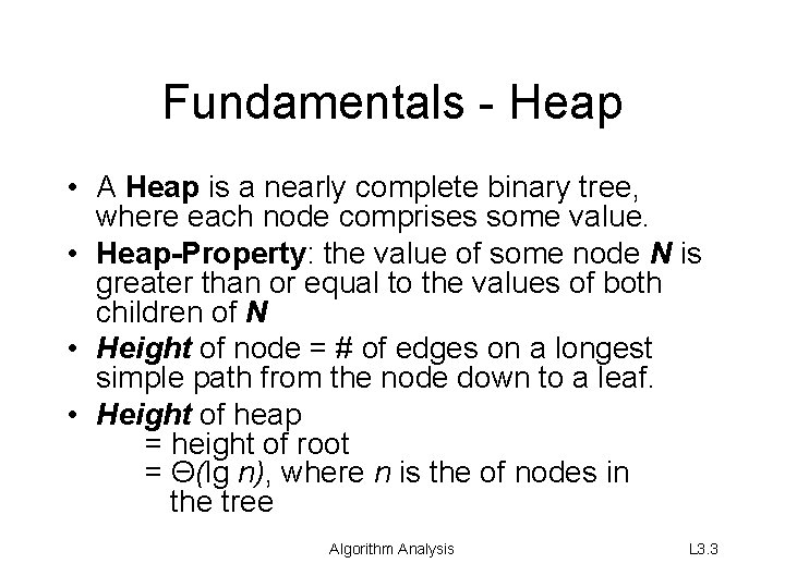
Fundamentals - Heap • A Heap is a nearly complete binary tree, where each node comprises some value. • Heap-Property: the value of some node N is greater than or equal to the values of both children of N • Height of node = # of edges on a longest simple path from the node down to a leaf. • Height of heap = height of root = Θ(lg n), where n is the of nodes in the tree Algorithm Analysis L 3. 3

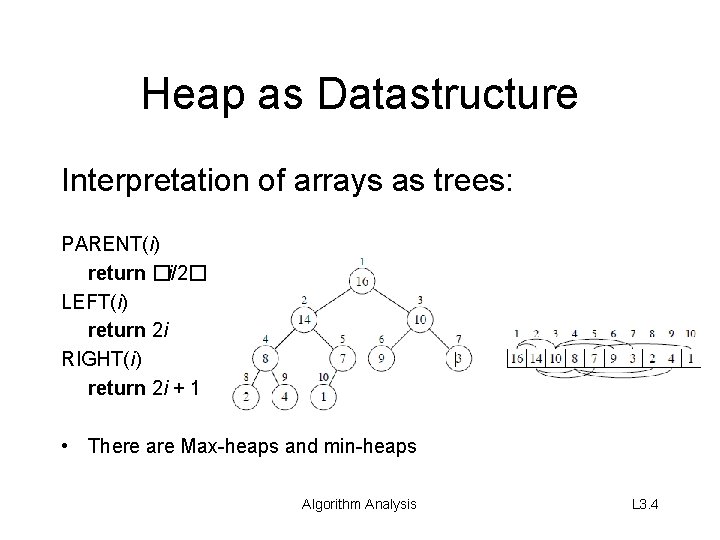
Heap as Datastructure Interpretation of arrays as trees: PARENT(i) return �i/2� LEFT(i) return 2 i RIGHT(i) return 2 i + 1 • There are Max-heaps and min-heaps Algorithm Analysis L 3. 4

MAX-HEAPIFY • MAX-HEAPIFY is used to maintain the max-heap property. – Before MAX-HEAPIFY, A[i] may be smaller than its children. – Assume left and right subtrees of i are maxheaps. – After MAX-HEAPIFY, subtree rooted at i is a max-heap. Algorithm Analysis L 3. 5

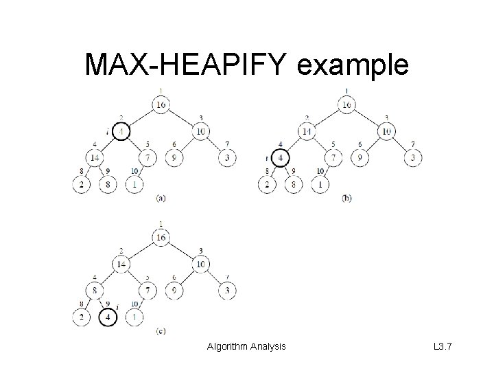
The way MAX-HEAPIFY works • Compare A[i ], A[LEFT(i )], and A[RIGHT(i )]. • If necessary, swap A[i ] with the larger of the two children to preserve heap property. • Continue this process of comparing and swapping down the heap, until subtree rooted at i is max-heap. If we hit a leaf, then the subtree rooted at the leaf is trivially a maxheap. Algorithm Analysis L 3. 6

MAX-HEAPIFY example Algorithm Analysis L 3. 7

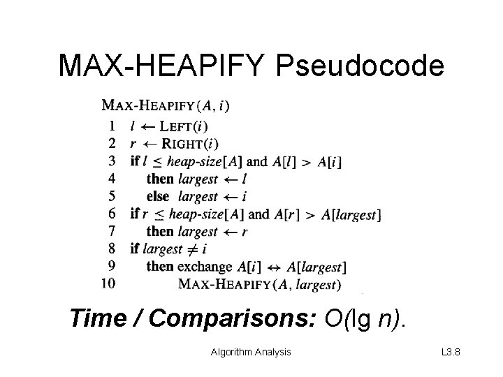
MAX-HEAPIFY Pseudocode Time / Comparisons: O(lg n). Algorithm Analysis L 3. 8

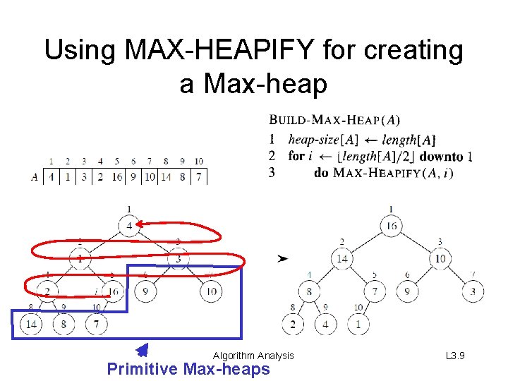
Using MAX-HEAPIFY for creating a Max-heap Algorithm Analysis Primitive Max-heaps L 3. 9

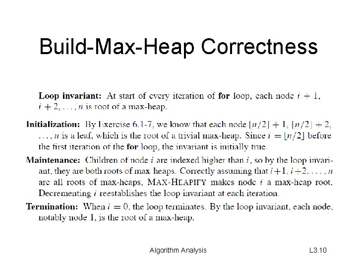
Build-Max-Heap Correctness Algorithm Analysis L 3. 10

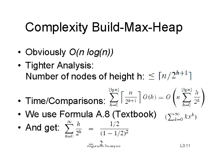
Complexity Build-Max-Heap • Obviously O(n log(n)) • Tighter Analysis: Number of nodes of height h: • Time/Comparisons: • We use Formula A. 8 (Textbook) • And get: Algorithm Analysis L 3. 11

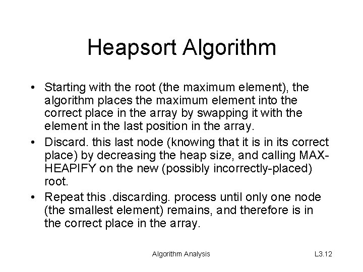
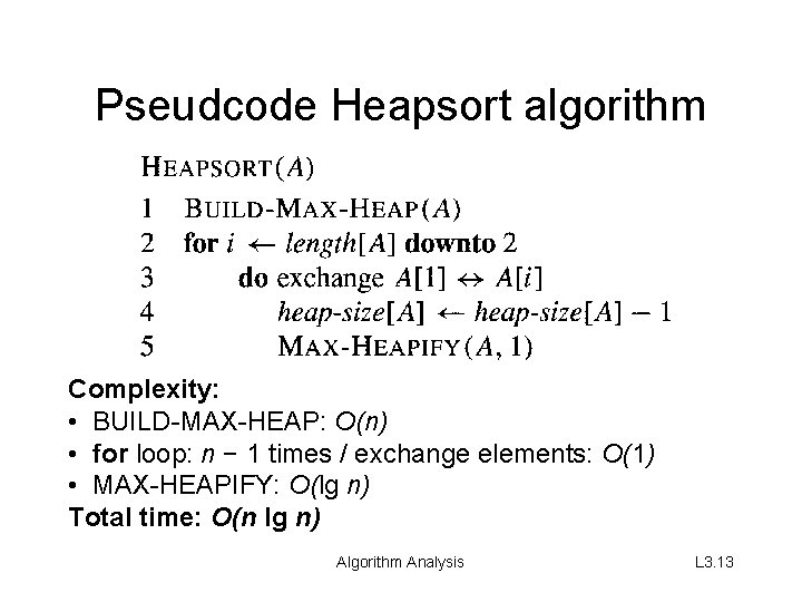
Heapsort Algorithm • Starting with the root (the maximum element), the algorithm places the maximum element into the correct place in the array by swapping it with the element in the last position in the array. • Discard. this last node (knowing that it is in its correct place) by decreasing the heap size, and calling MAXHEAPIFY on the new (possibly incorrectly-placed) root. • Repeat this. discarding. process until only one node (the smallest element) remains, and therefore is in the correct place in the array. Algorithm Analysis L 3. 12

Pseudcode Heapsort algorithm Complexity: • BUILD-MAX-HEAP: O(n) • for loop: n − 1 times / exchange elements: O(1) • MAX-HEAPIFY: O(lg n) Total time: O(n lg n) Algorithm Analysis L 3. 13

Priority Queues

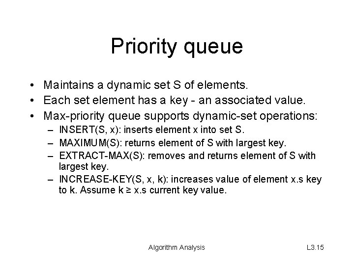
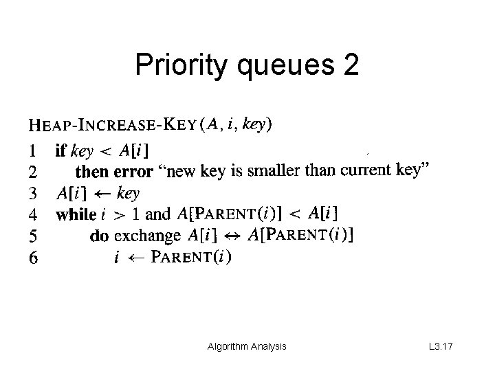
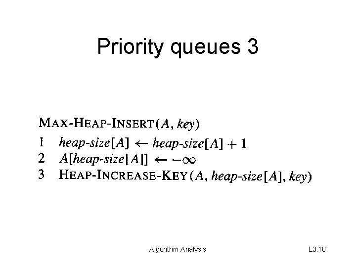
Priority queue • Maintains a dynamic set S of elements. • Each set element has a key - an associated value. • Max-priority queue supports dynamic-set operations: – INSERT(S, x): inserts element x into set S. – MAXIMUM(S): returns element of S with largest key. – EXTRACT-MAX(S): removes and returns element of S with largest key. – INCREASE-KEY(S, x, k): increases value of element x. s key to k. Assume k ≥ x. s current key value. Algorithm Analysis L 3. 15

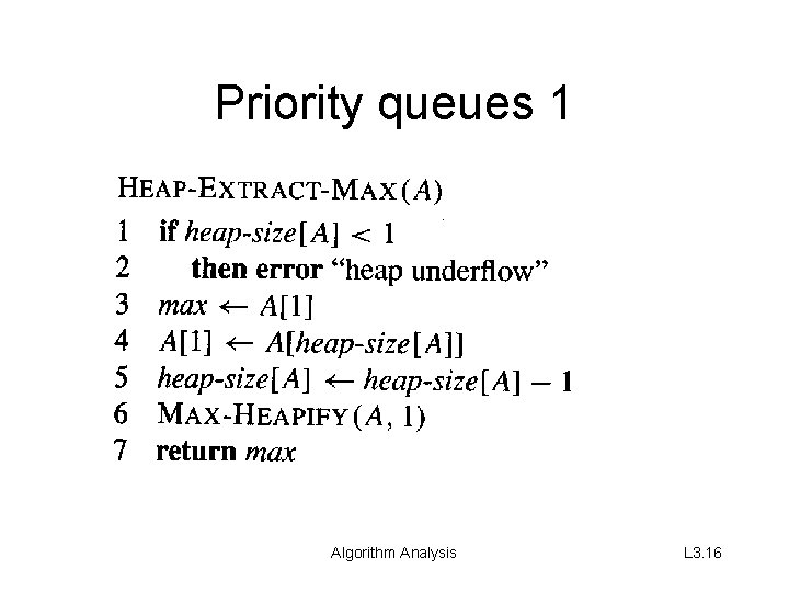
Priority queues 1 Algorithm Analysis L 3. 16

Priority queues 2 Algorithm Analysis L 3. 17

Priority queues 3 Algorithm Analysis L 3. 18

Quicksort

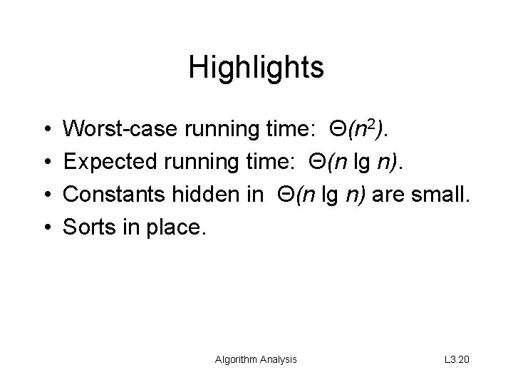
Highlights • • Worst-case running time: Θ(n 2). Expected running time: Θ(n lg n). Constants hidden in Θ(n lg n) are small. Sorts in place. Algorithm Analysis L 3. 20

Divide and Conquer Strategy with Quicksort • Divide: Partition A[p. . r ], into two (possibly empty) subarrays A[p. . q − 1] and A[q + 1. . r ], such that each element in the first subarray A[p. . q − 1] is ≤ A[q] and A[q] is ≤ each element in the second subarray A[q + 1. . r] • Conquer: Sort the two subarrays by recursive calls to QUICKSORT • Combine: No work is needed to combine the subarrays, because they are sorted in place. Algorithm Analysis L 3. 21

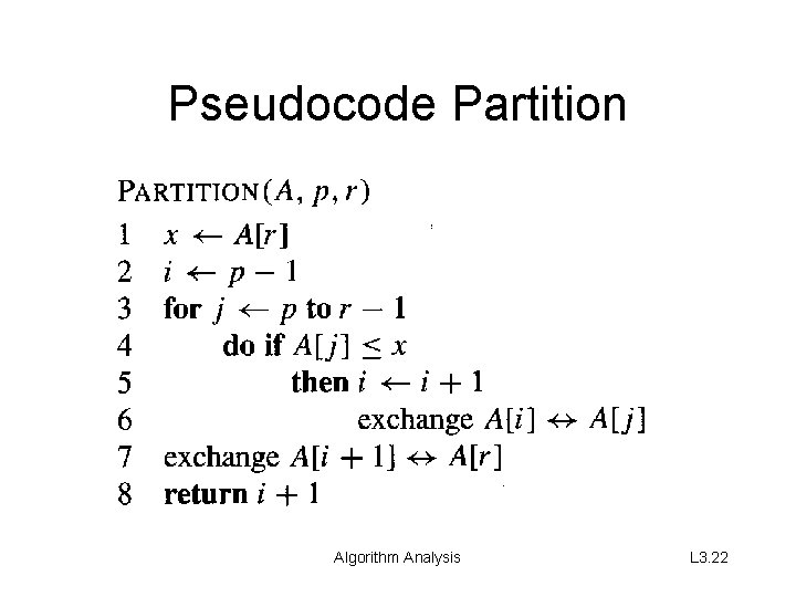
Pseudocode Partition Algorithm Analysis L 3. 22

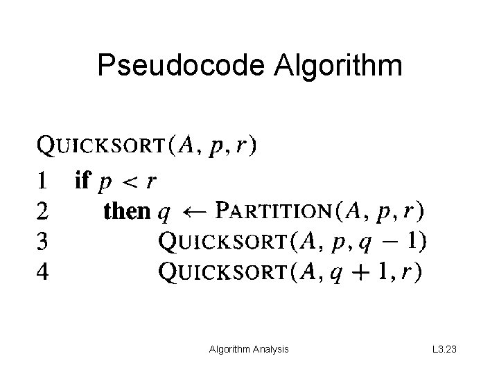
Pseudocode Algorithm Analysis L 3. 23

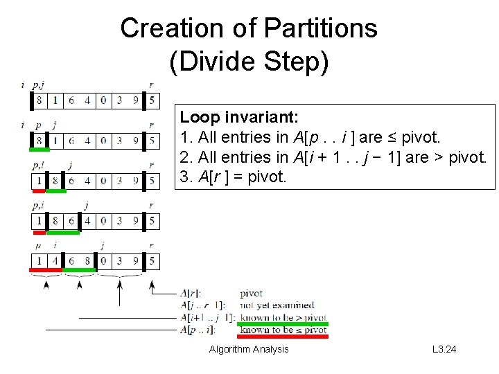
Creation of Partitions (Divide Step) Loop invariant: 1. All entries in A[p. . i ] are ≤ pivot. 2. All entries in A[i + 1. . j − 1] are > pivot. 3. A[r ] = pivot. Algorithm Analysis L 3. 24

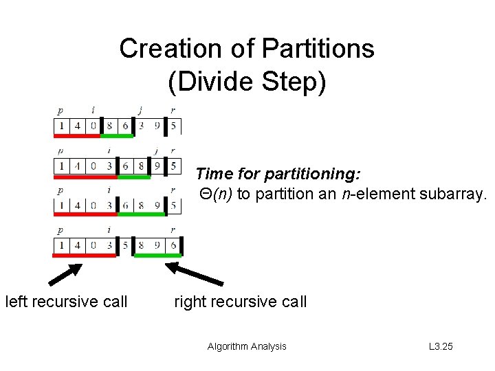
Creation of Partitions (Divide Step) Time for partitioning: Θ(n) to partition an n-element subarray. left recursive call right recursive call Algorithm Analysis L 3. 25

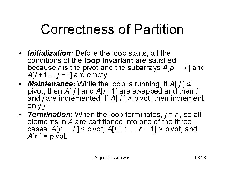
Correctness of Partition • Initialization: Before the loop starts, all the conditions of the loop invariant are satisfied, because r is the pivot and the subarrays A[p. . i ] and A[i +1. . j − 1] are empty. • Maintenance: While the loop is running, if A[ j ] ≤ pivot, then A[ j ] and A[i +1] are swapped and then i and j are incremented. If A[ j ] > pivot, then increment only j. • Termination: When the loop terminates, j = r , so all elements in A are partitioned into one of the three cases: A[p. . i ] ≤ pivot, A[i + 1. . r − 1] > pivot, and A[r ] = pivot. Algorithm Analysis L 3. 26

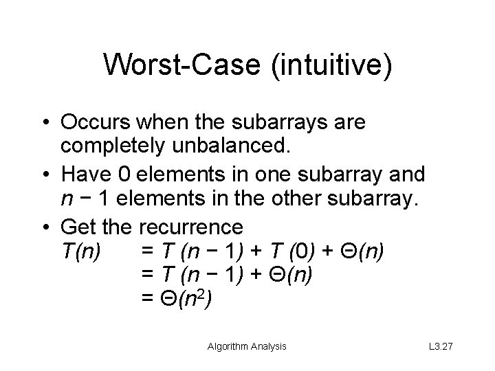
Worst-Case (intuitive) • Occurs when the subarrays are completely unbalanced. • Have 0 elements in one subarray and n − 1 elements in the other subarray. • Get the recurrence T(n) = T (n − 1) + T (0) + Θ(n) = T (n − 1) + Θ(n) = Θ(n 2) Algorithm Analysis L 3. 27

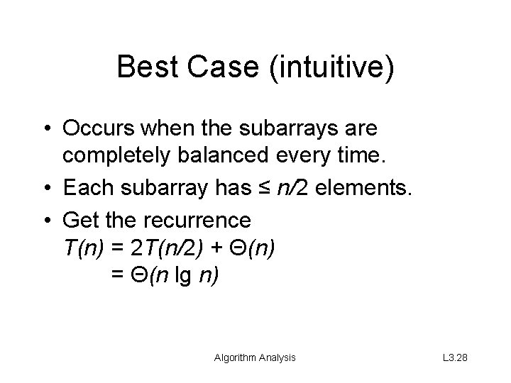
Best Case (intuitive) • Occurs when the subarrays are completely balanced every time. • Each subarray has ≤ n/2 elements. • Get the recurrence T(n) = 2 T(n/2) + Θ(n) = Θ(n lg n) Algorithm Analysis L 3. 28

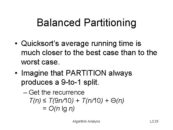
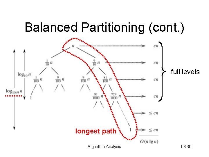
Balanced Partitioning • Quicksort’s average running time is much closer to the best case than to the worst case. • Imagine that PARTITION always produces a 9 -to-1 split. – Get the recurrence T(n) ≤ T(9 n/10) + T(n/10) + Θ(n) = O(n lg n) Algorithm Analysis L 3. 29

Balanced Partitioning (cont. ) full levels longest path Algorithm Analysis L 3. 30

Average Case (Intuition) • Splits in the recursion tree will not always be constant. • There will usually be a mix of good and bad splits throughout the recursion tree. • To see that this doesn’t affect the asymptotic running time of quicksort, assume that levels alternate between best-case and worst-case splits. Algorithm Analysis L 3. 31

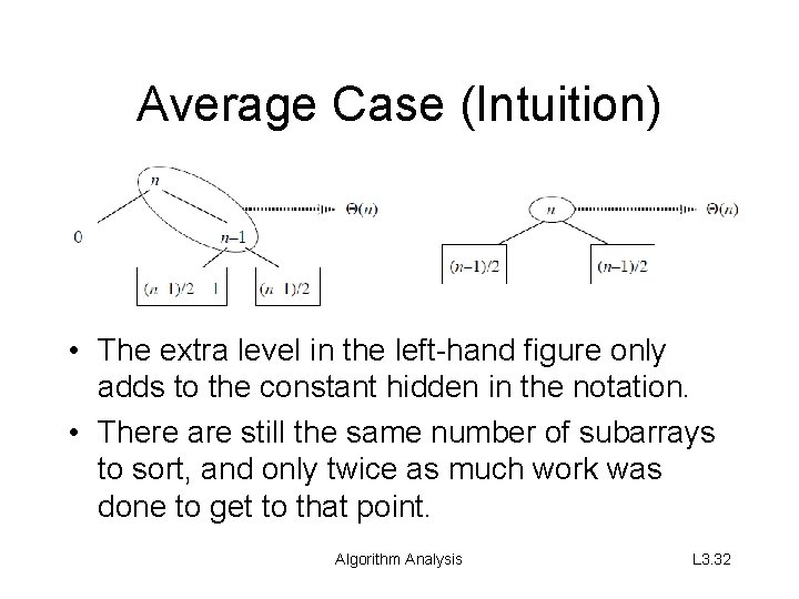
Average Case (Intuition) • The extra level in the left-hand figure only adds to the constant hidden in the notation. • There are still the same number of subarrays to sort, and only twice as much work was done to get to that point. Algorithm Analysis L 3. 32

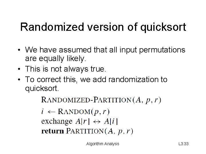
Randomized version of quicksort • We have assumed that all input permutations are equally likely. • This is not always true. • To correct this, we add randomization to quicksort. Algorithm Analysis L 3. 33

Average Case (Detailed) • The dominant cost of the algorithm is partitioning. • PARTITION removes the pivot element from future consideration each time. Thus, PARTITION is called at most n times. • The amount of work that each call to PARTITION does is a constant plus the number of comparisons that are performed in its for loop. • Let X = the total number of comparisons performed in all calls to PARTITION. So, total work done over the entire execution is O(n + X). . Algorithm Analysis L 3. 34

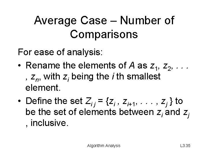
Average Case – Number of Comparisons For ease of analysis: • Rename the elements of A as z 1, z 2, . . . , zn, with zi being the i th smallest element. • Define the set Zi j = {zi , zi+1, . . . , zj } to be the set of elements between zi and zj , inclusive. Algorithm Analysis L 3. 35

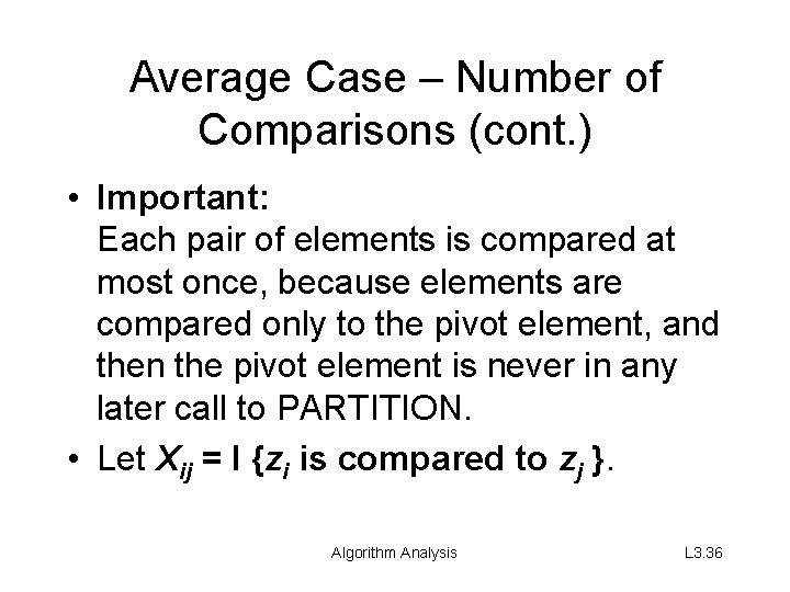
Average Case – Number of Comparisons (cont. ) • Important: Each pair of elements is compared at most once, because elements are compared only to the pivot element, and then the pivot element is never in any later call to PARTITION. • Let Xij = I {zi is compared to zj }. Algorithm Analysis L 3. 36

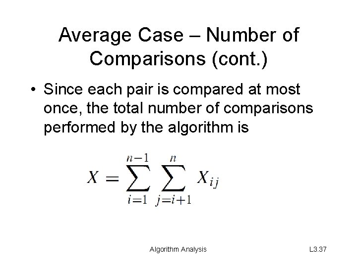
Average Case – Number of Comparisons (cont. ) • Since each pair is compared at most once, the total number of comparisons performed by the algorithm is Algorithm Analysis L 3. 37

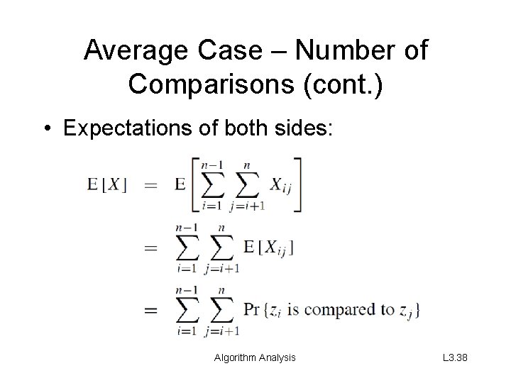
Average Case – Number of Comparisons (cont. ) • Expectations of both sides: Algorithm Analysis L 3. 38

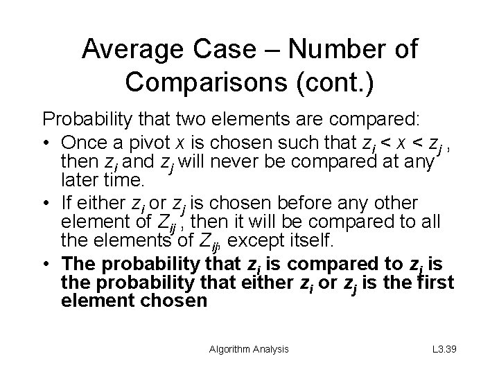
Average Case – Number of Comparisons (cont. ) Probability that two elements are compared: • Once a pivot x is chosen such that zi < x < zj , then zi and zj will never be compared at any later time. • If either zi or zj is chosen before any other element of Zij , then it will be compared to all the elements of Zij, except itself. • The probability that zi is compared to zj is the probability that either zi or zj is the first element chosen Algorithm Analysis L 3. 39

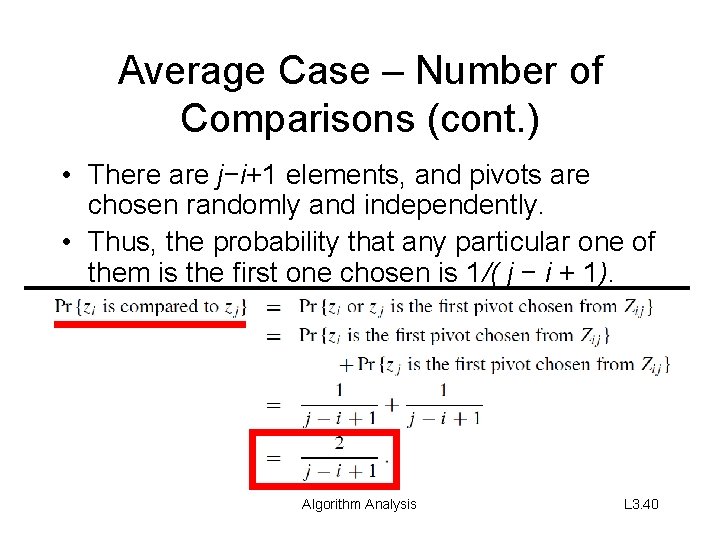
Average Case – Number of Comparisons (cont. ) • There are j−i+1 elements, and pivots are chosen randomly and independently. • Thus, the probability that any particular one of them is the first one chosen is 1/( j − i + 1). Algorithm Analysis L 3. 40

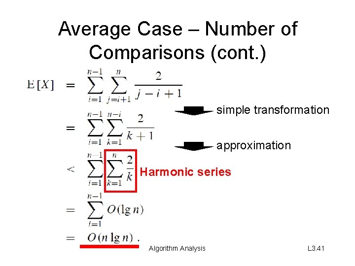
Average Case – Number of Comparisons (cont. ) simple transformation approximation Harmonic series Algorithm Analysis L 3. 41