Lecture 25 Algo Rhythm Design Techniques F Agenda

Lecture 25: Algo. Rhythm Design Techniques F Agenda for today’s class: í Coping with NP-complete and other hard problems ç Approximation using Greedy Techniques l Optimally bagging groceries: Bin Packing ç Divide & Conquer Algorithms and their Recurrences ç Dynamic Programming by “memoizing” l Fibonacci’s Revenge ç Randomized Data Structures and Algorithms l Treaps l “Probably correct” primality testing ç In the Sections on Thursday: Backtracking l Game Trees, minimax, and alpha-beta pruning F Read Chapter 10 and Sec 12. 5 in the textbook R. Rao, CSE 326 1

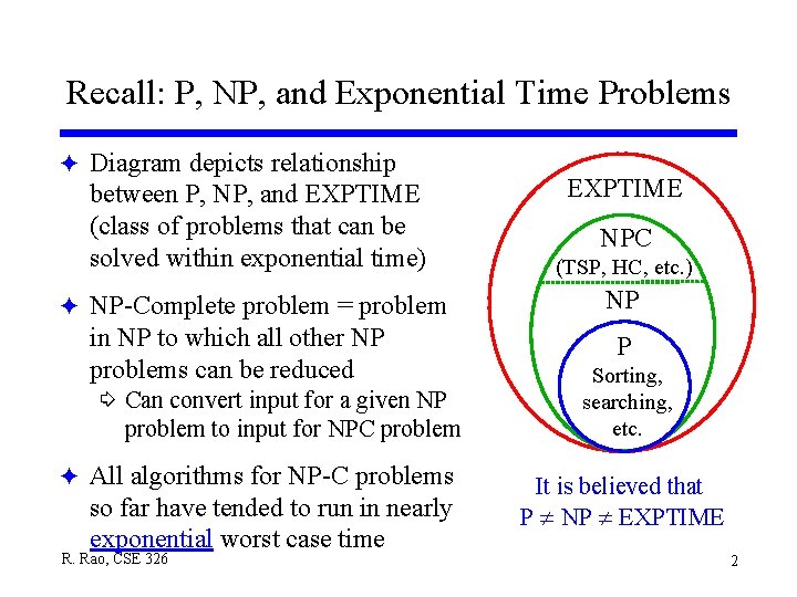
Recall: P, NP, and Exponential Time Problems F Diagram depicts relationship EXPTIME between P, NP, and EXPTIME (class of problems that can be solved within exponential time) (TSP, HC, etc. ) F NP-Complete problem = problem NP in NP to which all other NP problems can be reduced í Can convert input for a given NP problem to input for NPC problem F All algorithms for NP-C problems so far have tended to run in nearly exponential worst case time R. Rao, CSE 326 NPC P Sorting, searching, etc. It is believed that P NP EXPTIME 2

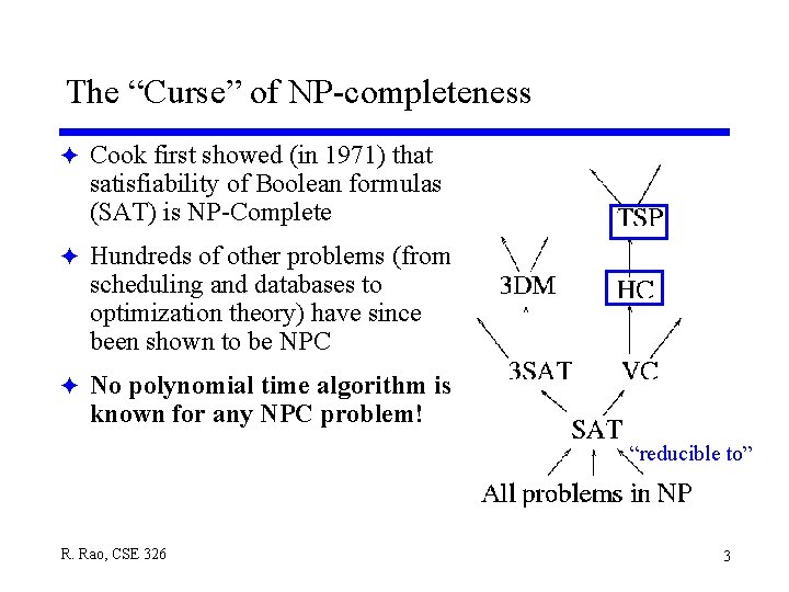
The “Curse” of NP-completeness F Cook first showed (in 1971) that satisfiability of Boolean formulas (SAT) is NP-Complete F Hundreds of other problems (from scheduling and databases to optimization theory) have since been shown to be NPC F No polynomial time algorithm is known for any NPC problem! “reducible to” R. Rao, CSE 326 3

Coping strategy #1: Greedy Approximations F Use a greedy algorithm to solve the given problem í Repeat until a solution is found: ç Among the set of possible next steps: Choose the current best-looking alternative and commit to it F Usually fast and simple F Works in some cases…(always finds optimal solutions) í Dijsktra’s single-source shortest path algorithm í Prim’s and Kruskal’s algorithm for finding MSTs F but not in others…(may find an approximate solution) í TSP – always choosing current least edge-cost node to visit next í Bagging groceries… R. Rao, CSE 326 4

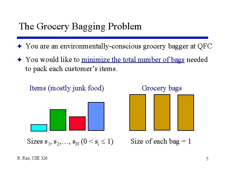
The Grocery Bagging Problem F You are an environmentally-conscious grocery bagger at QFC F You would like to minimize the total number of bags needed to pack each customer’s items. Items (mostly junk food) Sizes s 1, s 2, …, s. N (0 < si 1) R. Rao, CSE 326 Grocery bags Size of each bag = 1 5

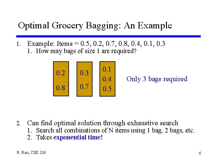
Optimal Grocery Bagging: An Example 1. Example: Items = 0. 5, 0. 2, 0. 7, 0. 8, 0. 4, 0. 1, 0. 3 1. How may bags of size 1 are required? 0. 2 0. 3 0. 8 0. 7 0. 1 0. 4 0. 5 Only 3 bags required 2. Can find optimal solution through exhaustive search 1. Search all combinations of N items using 1 bag, 2 bags, etc. 2. Takes exponential time! R. Rao, CSE 326 6

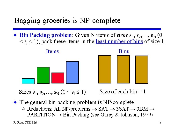
Bagging groceries is NP-complete F Bin Packing problem: Given N items of sizes s 1, s 2, …, s. N (0 < si 1), pack these items in the least number of bins of size 1. Items Bins Sizes s 1, s 2, …, s. N (0 < si 1) Size of each bin = 1 F The general bin packing problem is NP-complete í Reductions: All NP-problems SAT 3 DM PARTITION Bin Packing (see Garey & Johnson, 1979) R. Rao, CSE 326 7

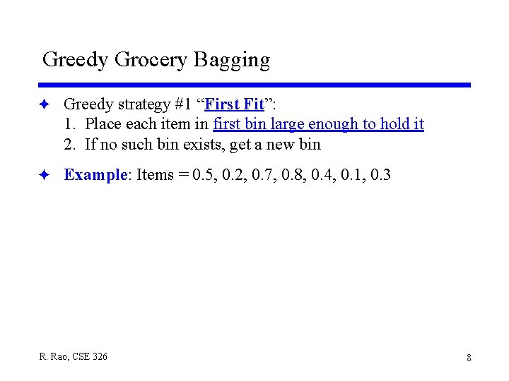
Greedy Grocery Bagging F Greedy strategy #1 “First Fit”: 1. Place each item in first bin large enough to hold it 2. If no such bin exists, get a new bin F Example: Items = 0. 5, 0. 2, 0. 7, 0. 8, 0. 4, 0. 1, 0. 3 R. Rao, CSE 326 8

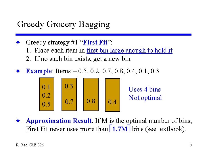
Greedy Grocery Bagging F Greedy strategy #1 “First Fit”: 1. Place each item in first bin large enough to hold it 2. If no such bin exists, get a new bin F Example: Items = 0. 5, 0. 2, 0. 7, 0. 8, 0. 4, 0. 1, 0. 3 0. 1 0. 2 0. 5 0. 3 0. 7 0. 8 0. 4 Uses 4 bins Not optimal F Approximation Result: If M is the optimal number of bins, First Fit never uses more than 1. 7 M bins (see textbook). R. Rao, CSE 326 9

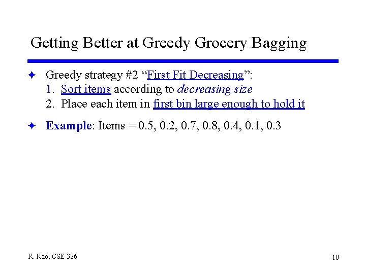
Getting Better at Greedy Grocery Bagging F Greedy strategy #2 “First Fit Decreasing”: 1. Sort items according to decreasing size 2. Place each item in first bin large enough to hold it F Example: Items = 0. 5, 0. 2, 0. 7, 0. 8, 0. 4, 0. 1, 0. 3 R. Rao, CSE 326 10

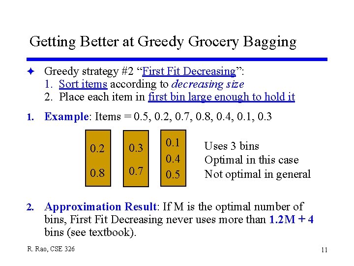
Getting Better at Greedy Grocery Bagging F Greedy strategy #2 “First Fit Decreasing”: 1. Sort items according to decreasing size 2. Place each item in first bin large enough to hold it 1. Example: Items = 0. 5, 0. 2, 0. 7, 0. 8, 0. 4, 0. 1, 0. 3 0. 2 0. 3 0. 8 0. 7 0. 1 0. 4 0. 5 Uses 3 bins Optimal in this case Not optimal in general 2. Approximation Result: If M is the optimal number of bins, First Fit Decreasing never uses more than 1. 2 M + 4 bins (see textbook). R. Rao, CSE 326 11

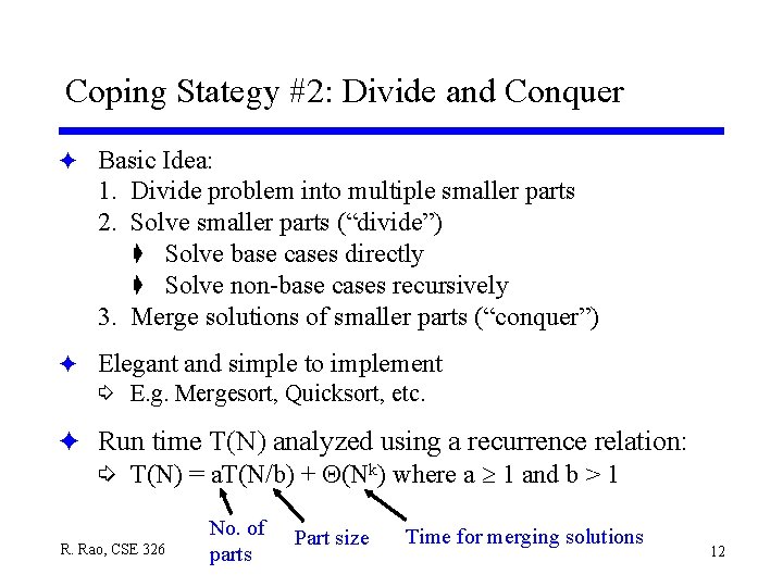
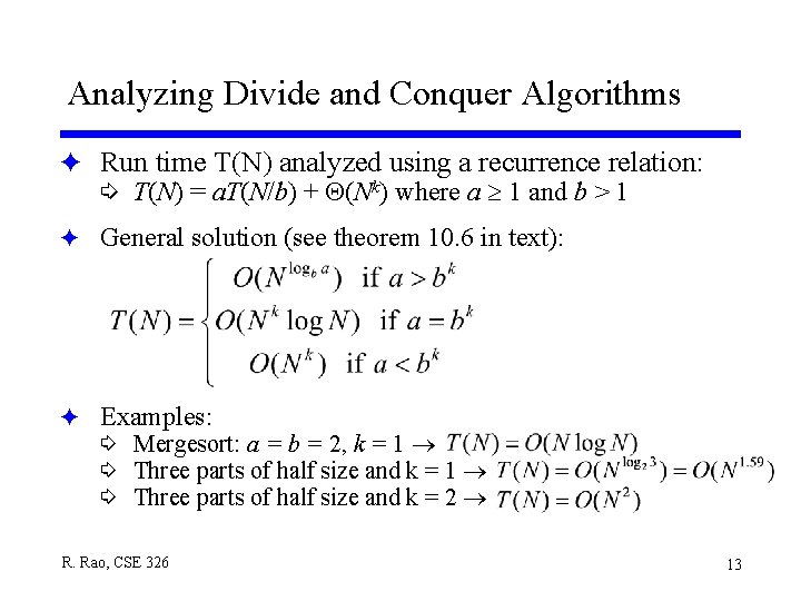
Coping Stategy #2: Divide and Conquer F Basic Idea: 1. Divide problem into multiple smaller parts 2. Solve smaller parts (“divide”) ç Solve base cases directly ç Solve non-base cases recursively 3. Merge solutions of smaller parts (“conquer”) F Elegant and simple to implement í E. g. Mergesort, Quicksort, etc. F Run time T(N) analyzed using a recurrence relation: í T(N) = a. T(N/b) + (Nk) where a 1 and b > 1 R. Rao, CSE 326 No. of parts Part size Time for merging solutions 12

Analyzing Divide and Conquer Algorithms F Run time T(N) analyzed using a recurrence relation: í T(N) = a. T(N/b) + (Nk) where a 1 and b > 1 F General solution (see theorem 10. 6 in text): F Examples: í Mergesort: a = b = 2, k = 1 í Three parts of half size and k = 2 R. Rao, CSE 326 13

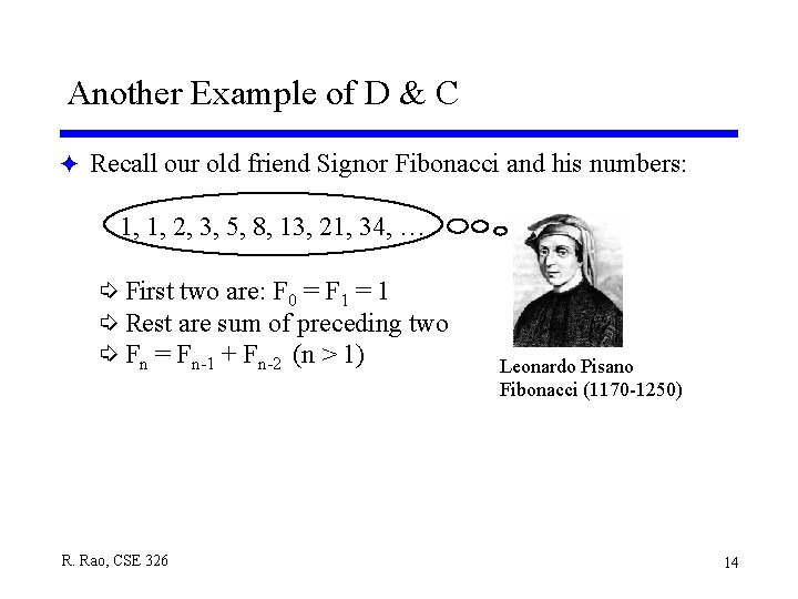
Another Example of D & C F Recall our old friend Signor Fibonacci and his numbers: 1, 1, 2, 3, 5, 8, 13, 21, 34, … í First two are: F 0 = F 1 = 1 í Rest are sum of preceding two í Fn = Fn-1 + Fn-2 (n > 1) R. Rao, CSE 326 Leonardo Pisano Fibonacci (1170 -1250) 14

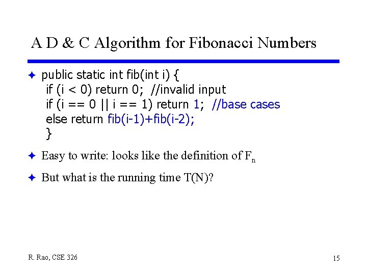
A D & C Algorithm for Fibonacci Numbers F public static int fib(int i) { if (i < 0) return 0; //invalid input if (i == 0 || i == 1) return 1; //base cases else return fib(i-1)+fib(i-2); } F Easy to write: looks like the definition of Fn F But what is the running time T(N)? R. Rao, CSE 326 15

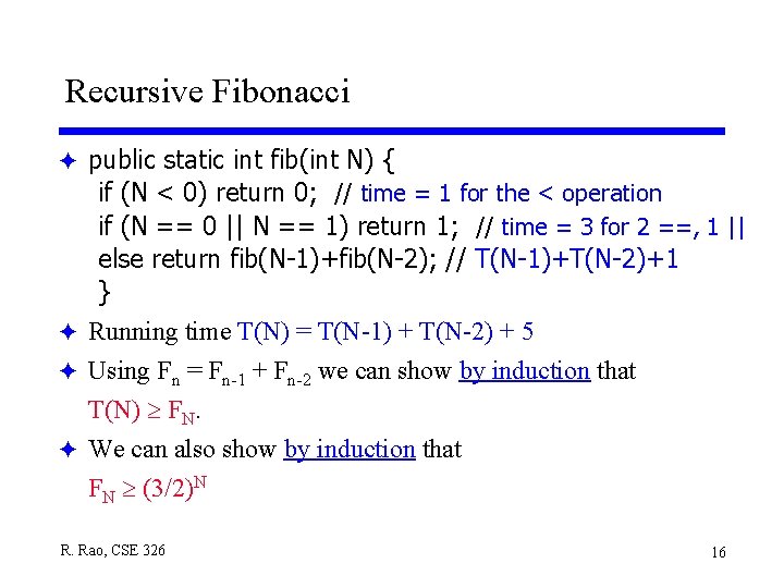
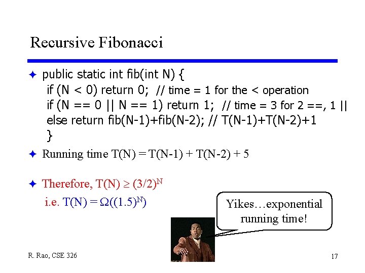
Recursive Fibonacci F public static int fib(int N) { if (N < 0) return 0; // time = 1 for the < operation if (N == 0 || N == 1) return 1; // time = 3 for 2 ==, 1 || else return fib(N-1)+fib(N-2); // T(N-1)+T(N-2)+1 } F Running time T(N) = T(N-1) + T(N-2) + 5 F Using Fn = Fn-1 + Fn-2 we can show by induction that T(N) FN. F We can also show by induction that FN (3/2)N R. Rao, CSE 326 16

Recursive Fibonacci F public static int fib(int N) { if (N < 0) return 0; // time = 1 for the < operation if (N == 0 || N == 1) return 1; // time = 3 for 2 ==, 1 || else return fib(N-1)+fib(N-2); // T(N-1)+T(N-2)+1 } F Running time T(N) = T(N-1) + T(N-2) + 5 F Therefore, T(N) (3/2)N i. e. T(N) = ((1. 5)N) R. Rao, CSE 326 Yikes…exponential running time! 17

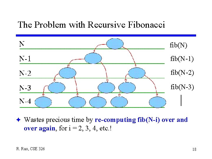
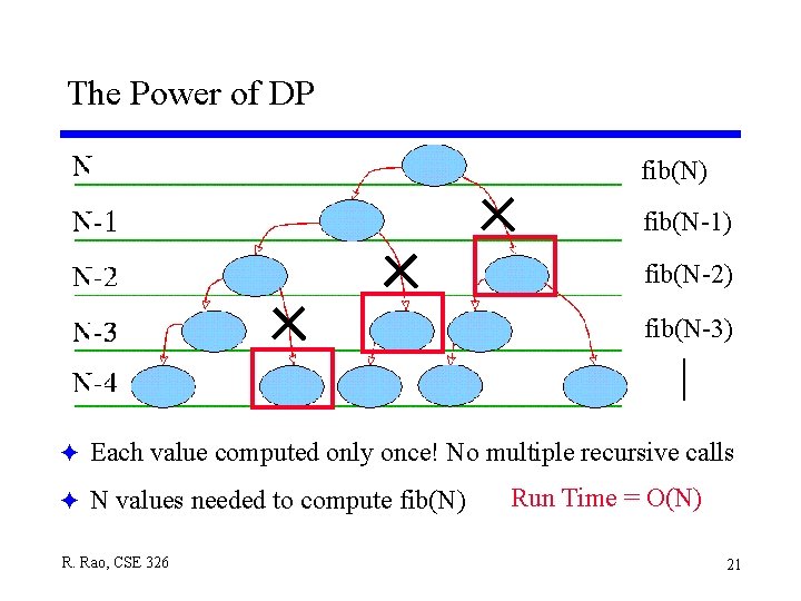
The Problem with Recursive Fibonacci fib(N) fib(N-1) fib(N-2) fib(N-3) F Wastes precious time by re-computing fib(N-i) over and over again, for i = 2, 3, 4, etc. ! R. Rao, CSE 326 18

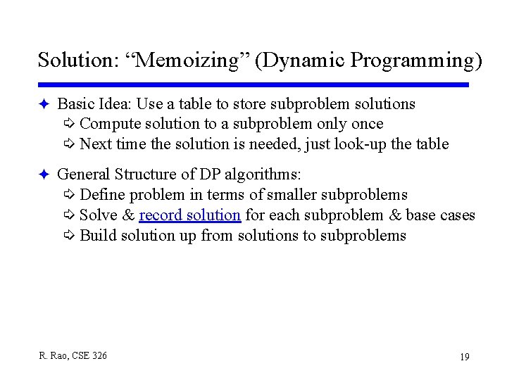
Solution: “Memoizing” (Dynamic Programming) F Basic Idea: Use a table to store subproblem solutions í Compute solution to a subproblem only once í Next time the solution is needed, just look-up the table F General Structure of DP algorithms: í Define problem in terms of smaller subproblems í Solve & record solution for each subproblem & base cases í Build solution up from solutions to subproblems R. Rao, CSE 326 19

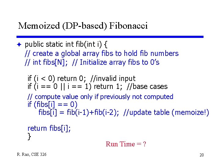
Memoized (DP-based) Fibonacci F public static int fib(int i) { // create a global array fibs to hold fib numbers // int fibs[N]; // Initialize array fibs to 0’s if (i < 0) return 0; //invalid input if (i == 0 || i == 1) return 1; //base cases // compute value only if previously not computed if (fibs[i] == 0) fibs[i] = fib(i-1)+fib(i-2); //update table (memoize!) return fibs[i]; } R. Rao, CSE 326 Run Time = ? 20

The Power of DP fib(N) fib(N-1) fib(N-2) fib(N-3) F Each value computed only once! No multiple recursive calls F N values needed to compute fib(N) R. Rao, CSE 326 Run Time = O(N) 21

Summary of Dynamic Programming F Very important technique in CS: Improves the run time of D & C algorithms whenever there are shared subproblems F Examples: í DP-based Fibonacci í Ordering matrix multiplications í Building optimal binary search trees í All-pairs shortest path í DNA sequence alignment í Optimal action-selection and reinforcement learning in robotics í etc. R. Rao, CSE 326 22

Coping Strategy #3: Viva Las Vegas! (Randomization) F Basic Idea: When faced with several alternatives, toss a coin and make a decision í Utilizes a pseudorandom number generator (Sec. 10. 4. 1 in text) F Example: Randomized Quick. Sort í Choose pivot randomly among array elements F Compared to choosing first element as pivot: í Worst case run time is O(N 2) in both cases ç Occurs if largest chosen as pivot at each stage í BUT: For same input, randomized algorithm most likely won’t repeat bad performance whereas deterministic quicksort will! í Expected run time for randomized quicksort is O(N log N) time for any input R. Rao, CSE 326 23

Randomized Data Structures F We’ve seen many data structures with good average case performance on random inputs, but bad behavior on particular inputs í E. g. Binary Search Trees F Instead of randomizing the input (which we cannot!), consider randomizing the data structure! R. Rao, CSE 326 24

What’s the Difference? F Deterministic data structure with good average time í If your application happens to always contain the “bad” inputs, you are in big trouble! F Randomized data structure with good expected time í Once in a while you will have an expensive operation, but no inputs can make this happen all the time F Kind of like an insurance policy for your algorithm! R. Rao, CSE 326 25

What’s the Difference? F Deterministic data structure with good average time í If your application happens to always contain the “bad” inputs, you are in big trouble! F Randomized data structure with good expected time í Once in a while you will have an expensive operation, but no inputs can make this happen all the time F Kind of like an insurance policy for your algorithm! R. Rao, CSE 326 (Disclaimer: Allstate wants nothing to do with this boring lecture or lecturer. ) 26

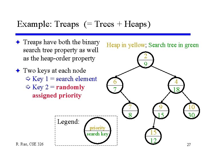
Example: Treaps (= Trees + Heaps) F Treaps have both the binary search tree property as well as the heap-order property Heap in yellow; Search tree in green 2 9 F Two keys at each node í Key 1 = search element í Key 2 = randomly assigned priority Legend: R. Rao, CSE 326 6 7 4 18 7 8 priority search key 9 15 15 12 10 30 27

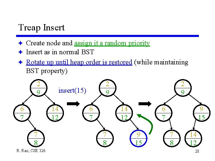
Treap Insert F Create node and assign it a random priority F Insert as in normal BST F Rotate up until heap order is restored (while maintaining BST property) 2 9 6 7 insert(15) 14 12 7 8 R. Rao, CSE 326 2 9 6 7 2 9 14 12 7 8 6 7 9 15 7 8 14 12 28

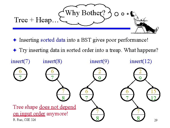
Why Bother? Tree + Heap… F Inserting sorted data into a BST gives poor performance! F Try inserting data in sorted order into a treap. What happens? insert(7) insert(8) insert(9) insert(12) 6 7 2 9 7 8 Tree shape does not depend on input order anymore! R. Rao, CSE 326 6 7 7 8 15 12 7 8 29

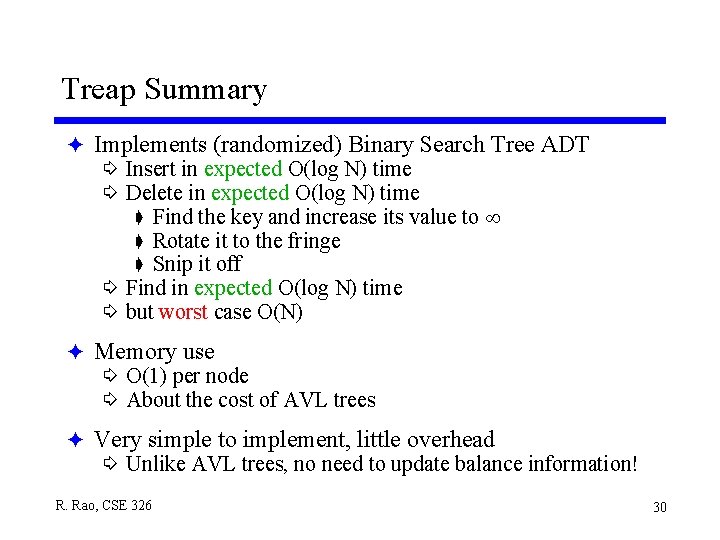
Treap Summary F Implements (randomized) Binary Search Tree ADT í Insert in expected O(log N) time í Delete in expected O(log N) time ç Find the key and increase its value to ç Rotate it to the fringe ç Snip it off í Find in expected O(log N) time í but worst case O(N) F Memory use í O(1) per node í About the cost of AVL trees F Very simple to implement, little overhead í Unlike AVL trees, no need to update balance information! R. Rao, CSE 326 30

Final Example: Randomized Primality Testing F Problem: Given a number N, is N prime? í Important for cryptography F F Randomized Algorithm based on a Result by Fermat: 1. Guess a random number A, 0 < A < N 2. If (AN-1 mod N) 1, then Output “N is not prime” 3. Otherwise, Output “N is (probably) prime” 1. N is prime with high probability but not 100% – N could be a “Carmichael number” – a slightly more complex test rules out this case (see text) – Can repeat steps 1 -3 to make error probability close to 0 Recent breakthrough: Polynomial time algorithm that is always correct (runs in O(log 12 N) time for input N) í Agrawal, M. , Kayal, N. , and Saxena, N. "Primes is in P. " Preprint, Aug. 6, 2002. http: //www. cse. iitk. ac. in/primality. pdf R. Rao, CSE 326 31

Yawn…are we done yet? To Do: Read Chapter 10 and Sec. 12. 5 (treaps) Finish HW assignment #5 Next Time: A Taste of Amortization Final Review R. Rao, CSE 326 32