Lecture 24 Process Scheduling Examples and for Realtime

Review: Categories of Process Scheduling • Batch Systems (Compute Servers) – Many processes, not

Scheduling Algorithm Goals • All Systems – Fairness – giving each process a fair

Review: Scheduling Algorithms for Batch Systems • First come first serve • Shortest job

Review: Scheduling Algorithms for Interactive Systems • • Round-Robin scheduling Priority scheduling Multiple queues

FCFS Arrival time CPU burst 0 P 1: 4 36 8 112 1 13

FCFS Time next ready 40 0 P 1: 4 36 8 112 1 76

RR, Q = 10 Arrival time CPU burst 0 P 1: 4 36 8

Real-time Scheduling • Definition – Systems whose correctness depends on their temporal aspects as

Real-time Scheduling Released Execution time Relative deadline Absolute deadline

Deadlines: Hard vs. Soft • Hard deadline – Disastrous or very serious consequences may

RM (Rate Monotonic) • • Optimal static-priority scheduling It assigns priority according to period

EDF (Earliest Deadline First) • Optimal dynamic priority scheduling • A task with a

Slides: 24

Download presentation

Lecture 24: Process Scheduling Examples and for Real-time Systems

Review: Categories of Process Scheduling • Batch Systems (Compute Servers) – Many processes, not interactive, throughput is important • Interactive Systems – PC • Real Time Systems – Guaranteed response times, meet deadlines

Scheduling Algorithm Goals • All Systems – Fairness – giving each process a fair share of the CPU – Policy enforcement – seeing that stated policy is carried out – Balance – keeping all parts of the system busy

Review: Scheduling Algorithms for Batch Systems • First come first serve • Shortest job first • Shortest remaining time next

Review: Scheduling Algorithms for Interactive Systems • • Round-Robin scheduling Priority scheduling Multiple queues Lottery scheduling

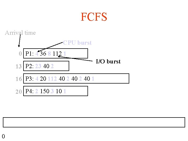
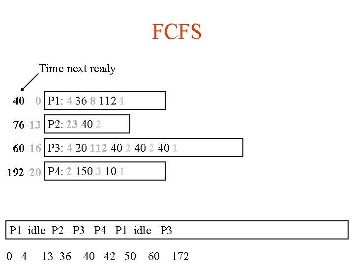
FCFS Arrival time CPU burst 0 P 1: 4 36 8 112 1 13 P 2: 23 40 2 16 P 3: 4 20 112 40 1 20 P 4: 2 150 3 10 1 0 I/O burst

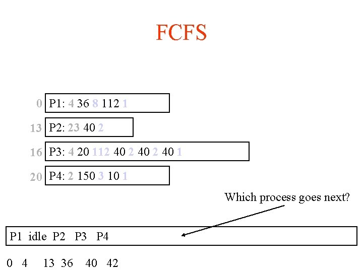
FCFS 0 P 1: 4 36 8 112 1 13 P 2: 23 40 2 16 P 3: 4 20 112 40 1 20 P 4: 2 150 3 10 1 Which process goes next? P 1 idle P 2 P 3 P 4 0 4 13 36 40 42

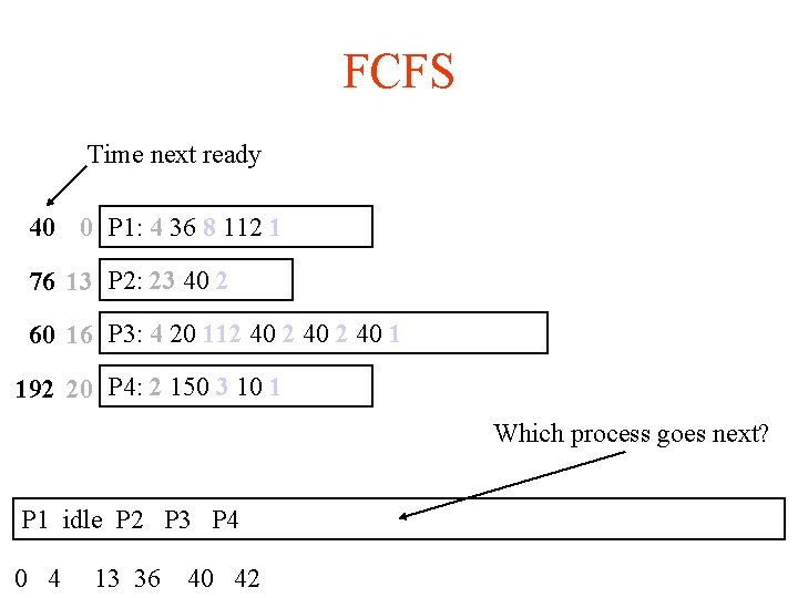
FCFS Time next ready 40 0 P 1: 4 36 8 112 1 76 13 P 2: 23 40 2 60 16 P 3: 4 20 112 40 1 192 20 P 4: 2 150 3 10 1 Which process goes next? P 1 idle P 2 P 3 P 4 0 4 13 36 40 42

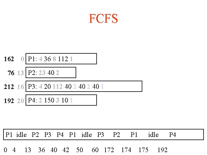
FCFS Time next ready 40 0 P 1: 4 36 8 112 1 76 13 P 2: 23 40 2 60 16 P 3: 4 20 112 40 1 192 20 P 4: 2 150 3 10 1 P 1 idle P 2 P 3 P 4 P 1 idle P 3 0 4 13 36 40 42 50 60 172

FCFS 162 0 P 1: 4 36 8 112 1 76 13 P 2: 23 40 2 212 16 P 3: 4 20 112 40 1 192 20 P 4: 2 150 3 10 1 P 1 idle P 2 P 3 P 4 P 1 idle P 3 0 4 13 36 40 42 50 P 2 60 172 P 1 174 idle 175 192 P 4

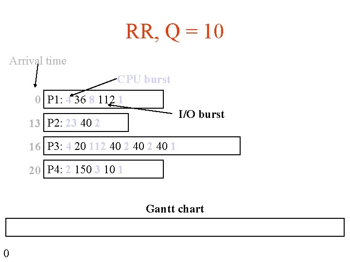
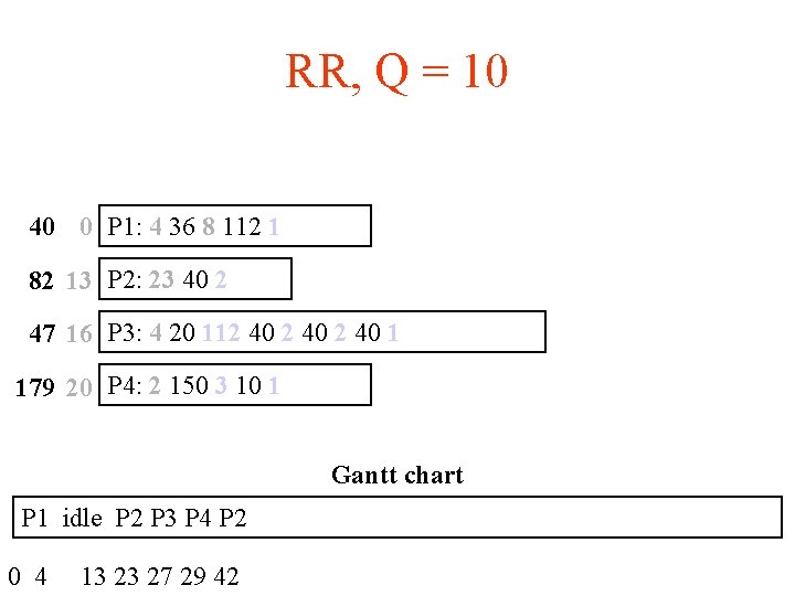
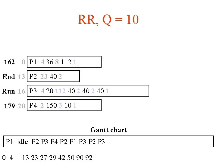
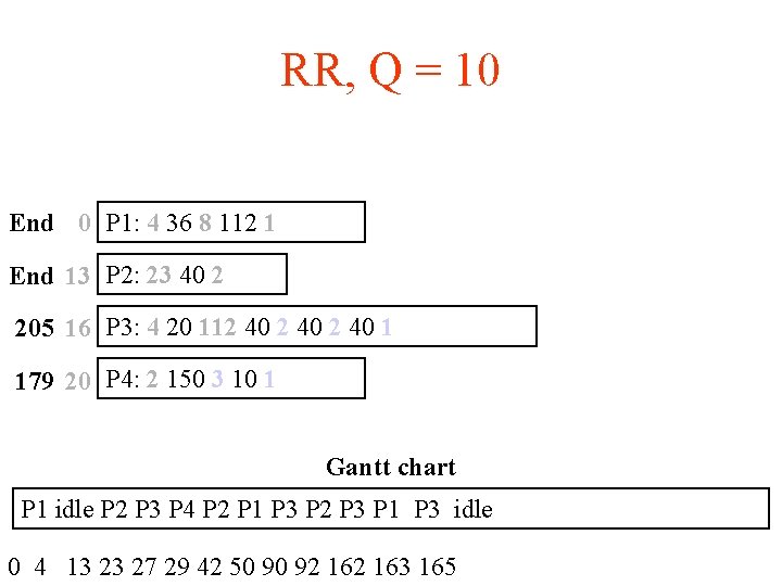
RR, Q = 10 Arrival time CPU burst 0 P 1: 4 36 8 112 1 I/O burst 13 P 2: 23 40 2 16 P 3: 4 20 112 40 1 20 P 4: 2 150 3 10 1 Gantt chart 0

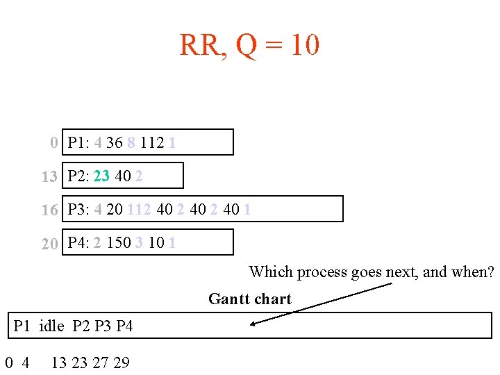
RR, Q = 10 0 P 1: 4 36 8 112 1 13 P 2: 23 40 2 16 P 3: 4 20 112 40 1 20 P 4: 2 150 3 10 1 Which process goes next, and when? Gantt chart P 1 idle P 2 P 3 P 4 0 4 13 23 27 29

RR, Q = 10 40 0 P 1: 4 36 8 112 1 82 13 P 2: 23 40 2 47 16 P 3: 4 20 112 40 1 179 20 P 4: 2 150 3 10 1 Gantt chart P 1 idle P 2 P 3 P 4 P 2 0 4 13 23 27 29 42

RR, Q = 10 162 0 P 1: 4 36 8 112 1 End 13 P 2: 23 40 2 Run 16 P 3: 4 20 112 40 1 179 20 P 4: 2 150 3 10 1 Gantt chart P 1 idle P 2 P 3 P 4 P 2 P 1 P 3 P 2 P 3 0 4 13 23 27 29 42 50 90 92

RR, Q = 10 End 0 P 1: 4 36 8 112 1 End 13 P 2: 23 40 2 205 16 P 3: 4 20 112 40 1 179 20 P 4: 2 150 3 10 1 Gantt chart P 1 idle P 2 P 3 P 4 P 2 P 1 P 3 P 2 P 3 P 1 P 3 idle 0 4 13 23 27 29 42 50 90 92 163 165

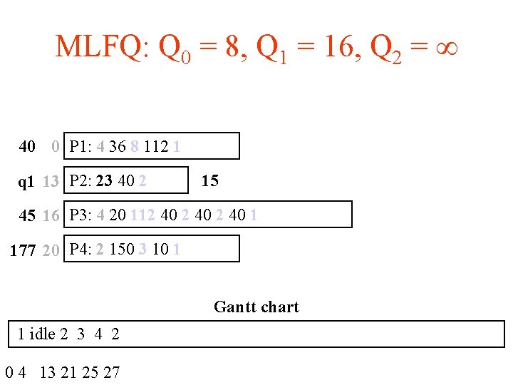
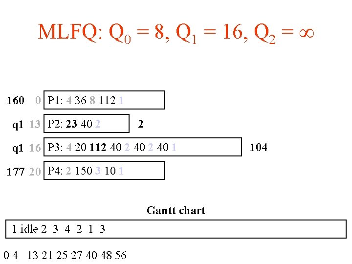
MLFQ: Q 0 = 8, Q 1 = 16, Q 2 = 40 0 P 1: 4 36 8 112 1 q 1 13 P 2: 23 40 2 15 45 16 P 3: 4 20 112 40 1 177 20 P 4: 2 150 3 10 1 Gantt chart 1 idle 2 3 4 2 0 4 13 21 25 27

MLFQ: Q 0 = 8, Q 1 = 16, Q 2 = 160 0 P 1: 4 36 8 112 1 q 1 13 P 2: 23 40 2 2 q 1 16 P 3: 4 20 112 40 1 177 20 P 4: 2 150 3 10 1 Gantt chart 1 idle 2 3 4 2 1 3 0 4 13 21 25 27 40 48 56 104

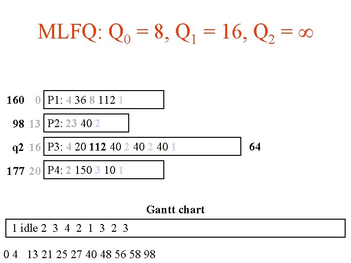
MLFQ: Q 0 = 8, Q 1 = 16, Q 2 = 160 0 P 1: 4 36 8 112 1 98 13 P 2: 23 40 2 q 2 16 P 3: 4 20 112 40 1 177 20 P 4: 2 150 3 10 1 Gantt chart 1 idle 2 3 4 2 1 3 2 3 0 4 13 21 25 27 40 48 56 58 98 64

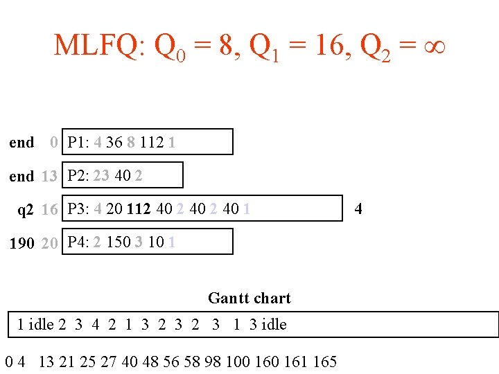
MLFQ: Q 0 = 8, Q 1 = 16, Q 2 = end 0 P 1: 4 36 8 112 1 end 13 P 2: 23 40 2 q 2 16 P 3: 4 20 112 40 1 190 20 P 4: 2 150 3 10 1 Gantt chart 1 idle 2 3 4 2 1 3 2 3 1 3 idle 0 4 13 21 25 27 40 48 56 58 98 100 161 165 4

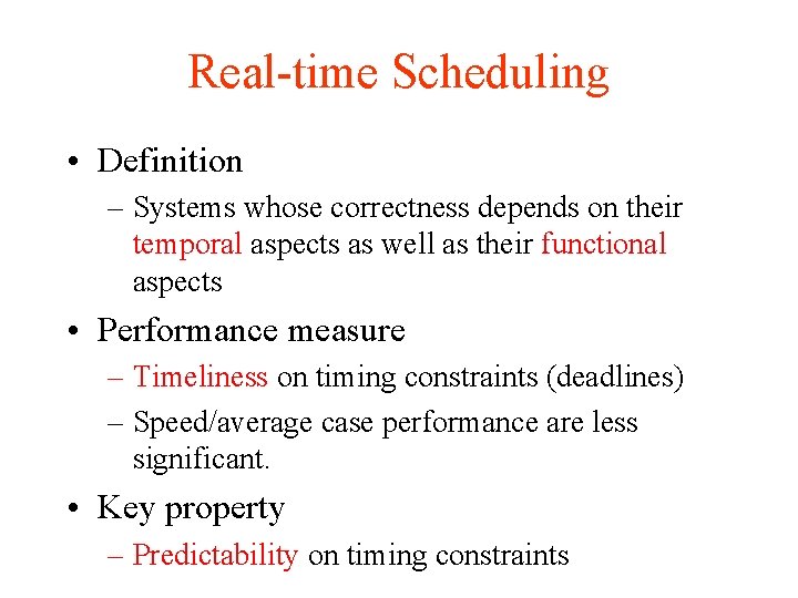
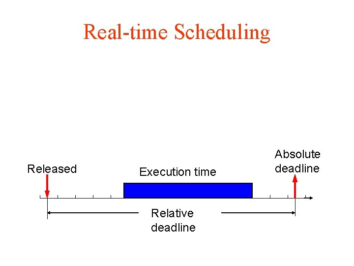
Real-time Scheduling • Definition – Systems whose correctness depends on their temporal aspects as well as their functional aspects • Performance measure – Timeliness on timing constraints (deadlines) – Speed/average case performance are less significant. • Key property – Predictability on timing constraints

Real-time Scheduling Released Execution time Relative deadline Absolute deadline

Deadlines: Hard vs. Soft • Hard deadline – Disastrous or very serious consequences may occur if the deadline is missed – Validation is essential : can all the deadlines be met, even under worst-case scenario? – Deterministic guarantees • Soft deadline – Ideally, the deadline should be met for maximum performance. The performance degrades in case of deadline misses. – Best effort approaches / statistical guarantees

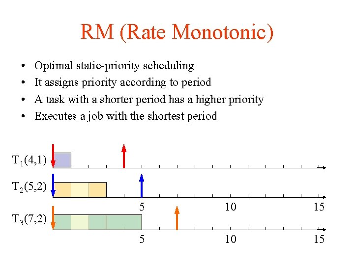
RM (Rate Monotonic) • • Optimal static-priority scheduling It assigns priority according to period A task with a shorter period has a higher priority Executes a job with the shortest period T 1 (4, 1) T 2 (5, 2) T 3 (7, 2) 5 10 15

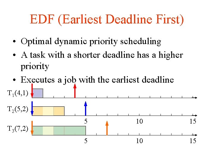
EDF (Earliest Deadline First) • Optimal dynamic priority scheduling • A task with a shorter deadline has a higher priority • Executes a job with the earliest deadline T 1 (4, 1) T 2 (5, 2) T 3 (7, 2) 5 10 15