Lecture 20 Support Vector Machines SVMs CS 109

Lecture 20: Support Vector Machines (SVMs) CS 109 A Introduction to Data Science Pavlos Protopapas and Kevin Rader

Outline • Classifying Linear Separable Data • Classifying Linear Non-Separable Data • Kernel Trick Text Reading: Ch. 9, p. 337 -356 CS 109 A, PROTOPAPAS, RADER 2

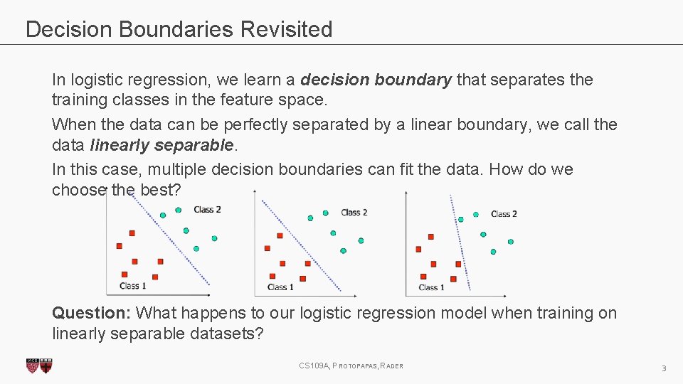
Decision Boundaries Revisited In logistic regression, we learn a decision boundary that separates the training classes in the feature space. When the data can be perfectly separated by a linear boundary, we call the data linearly separable. In this case, multiple decision boundaries can fit the data. How do we choose the best? Question: What happens to our logistic regression model when training on linearly separable datasets? CS 109 A, PROTOPAPAS, RADER 3

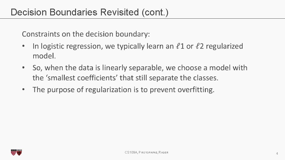
Decision Boundaries Revisited (cont. ) CS 109 A, PROTOPAPAS, RADER 4

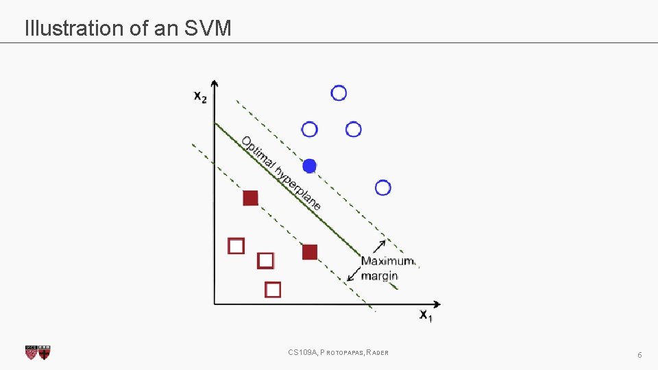
Decision Boundaries Revisited (cont. ) Constraints on the decision boundary: • We can consider alternative constraints that prevent overfitting. • For example, we may prefer a decision boundary that does not ‘favor’ any class (esp. when the classes are roughly equally populous). • Geometrically, this means choosing a boundary that maximizes the distance or margin between the boundary and both classes. CS 109 A, PROTOPAPAS, RADER 5

Illustration of an SVM CS 109 A, PROTOPAPAS, RADER 6

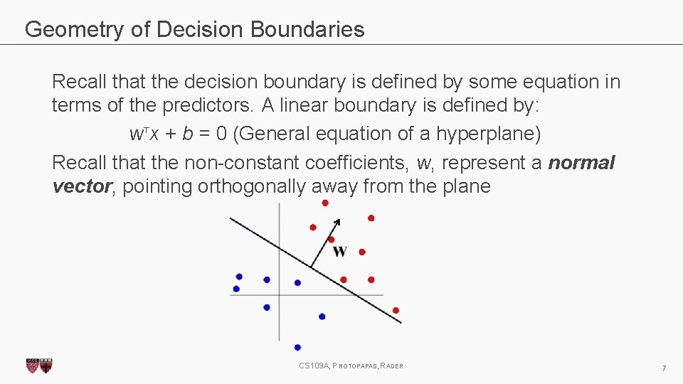
Geometry of Decision Boundaries Recall that the decision boundary is defined by some equation in terms of the predictors. A linear boundary is defined by: w⊤x + b = 0 (General equation of a hyperplane) Recall that the non-constant coefficients, w, represent a normal vector, pointing orthogonally away from the plane CS 109 A, PROTOPAPAS, RADER 7

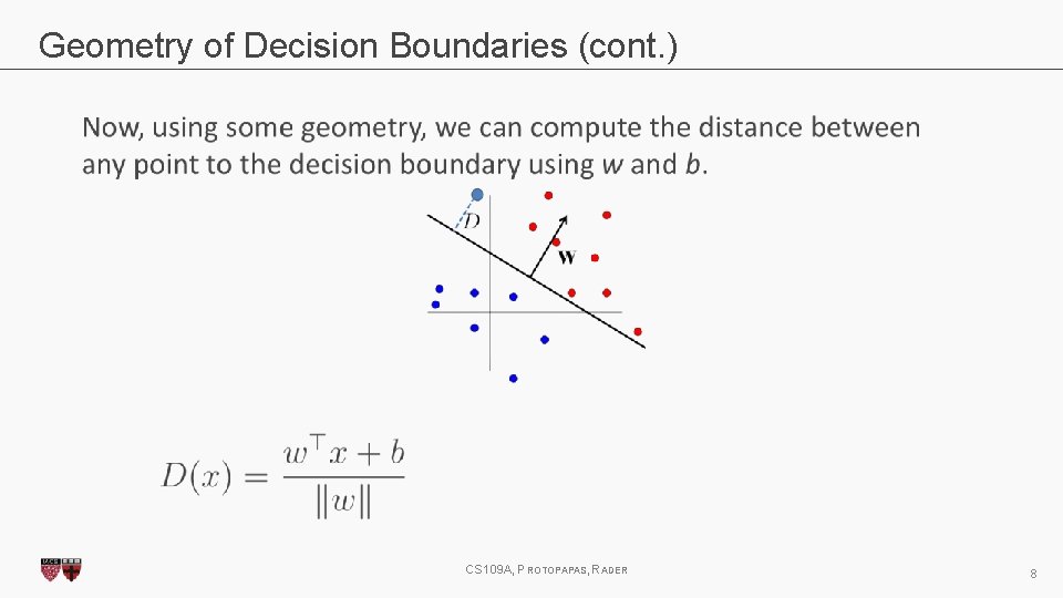
Geometry of Decision Boundaries (cont. ) CS 109 A, PROTOPAPAS, RADER 8

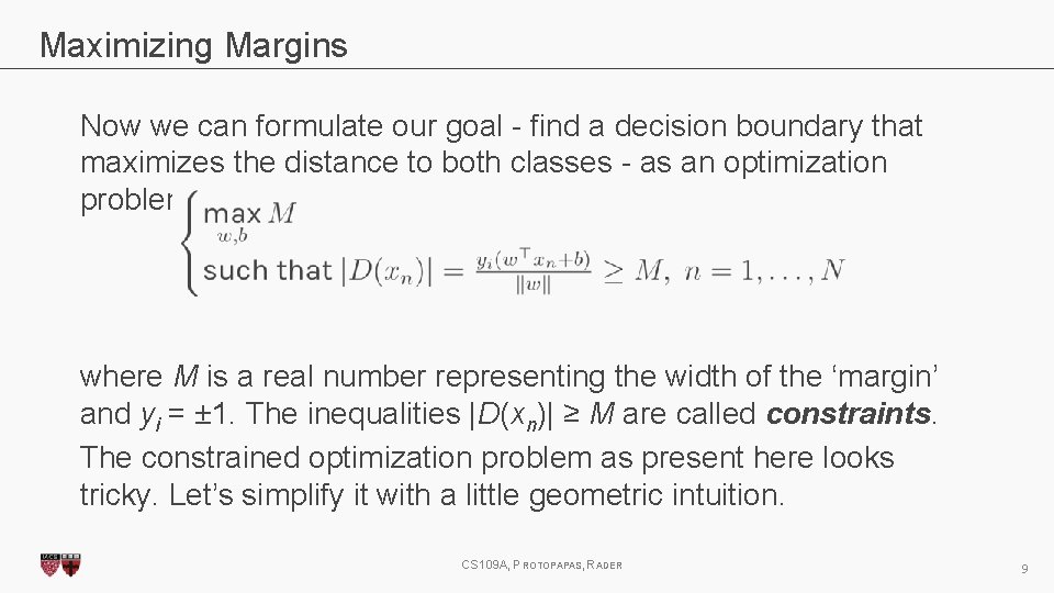
Maximizing Margins Now we can formulate our goal - find a decision boundary that maximizes the distance to both classes - as an optimization problem: where M is a real number representing the width of the ‘margin’ and yi = ± 1. The inequalities |D(xn)| ≥ M are called constraints. The constrained optimization problem as present here looks tricky. Let’s simplify it with a little geometric intuition. CS 109 A, PROTOPAPAS, RADER 9

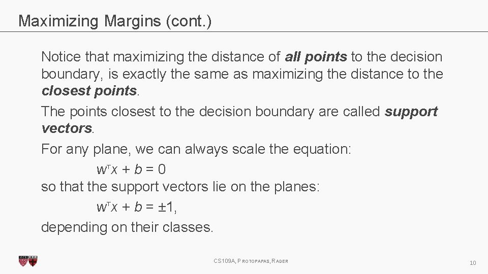
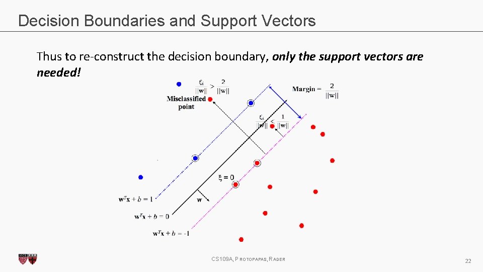
Maximizing Margins (cont. ) Notice that maximizing the distance of all points to the decision boundary, is exactly the same as maximizing the distance to the closest points. The points closest to the decision boundary are called support vectors. For any plane, we can always scale the equation: w ⊤x + b = 0 so that the support vectors lie on the planes: w⊤x + b = ± 1, depending on their classes. CS 109 A, PROTOPAPAS, RADER 10

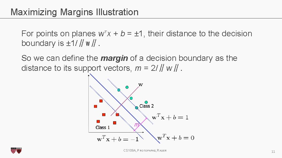
Maximizing Margins Illustration For points on planes w⊤x + b = ± 1, their distance to the decision boundary is ± 1/∥w∥. So we can define the margin of a decision boundary as the distance to its support vectors, m = 2/∥w∥. CS 109 A, PROTOPAPAS, RADER 11

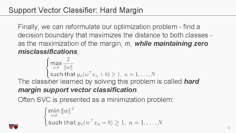
Support Vector Classifier: Hard Margin Finally, we can reformulate our optimization problem - find a decision boundary that maximizes the distance to both classes as the maximization of the margin, m, while maintaining zero misclassifications, The classifier learned by solving this problem is called hard margin support vector classification. Often SVC is presented as a minimization problem: CS 109 A, PROTOPAPAS, RADER 12

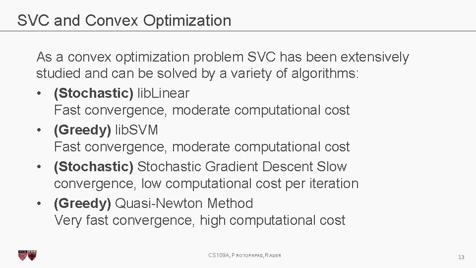
SVC and Convex Optimization As a convex optimization problem SVC has been extensively studied and can be solved by a variety of algorithms: • (Stochastic) lib. Linear Fast convergence, moderate computational cost • (Greedy) lib. SVM Fast convergence, moderate computational cost • (Stochastic) Stochastic Gradient Descent Slow convergence, low computational cost per iteration • (Greedy) Quasi-Newton Method Very fast convergence, high computational cost CS 109 A, PROTOPAPAS, RADER 13

Classifying Linear Non-Separable Data CS 109 A, PROTOPAPAS, RADER 14

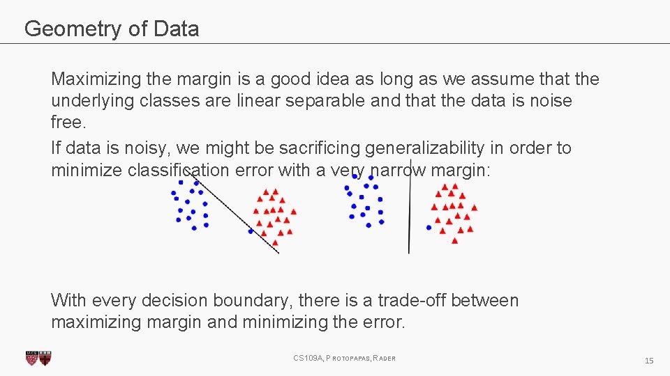
Geometry of Data Maximizing the margin is a good idea as long as we assume that the underlying classes are linear separable and that the data is noise free. If data is noisy, we might be sacrificing generalizability in order to minimize classification error with a very narrow margin: With every decision boundary, there is a trade-off between maximizing margin and minimizing the error. CS 109 A, PROTOPAPAS, RADER 15

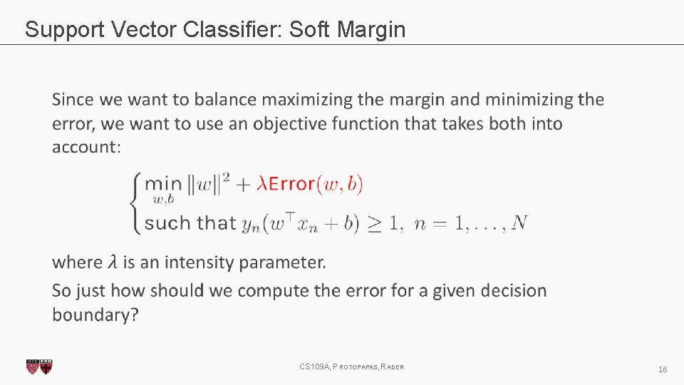
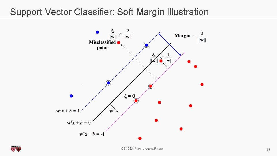
Support Vector Classifier: Soft Margin CS 109 A, PROTOPAPAS, RADER 16

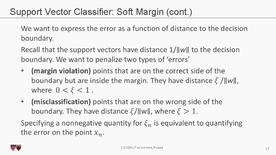
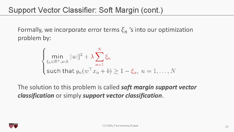
Support Vector Classifier: Soft Margin (cont. ) CS 109 A, PROTOPAPAS, RADER 17

Support Vector Classifier: Soft Margin Illustration CS 109 A, PROTOPAPAS, RADER 18

Support Vector Classifier: Soft Margin (cont. ) CS 109 A, PROTOPAPAS, RADER 19

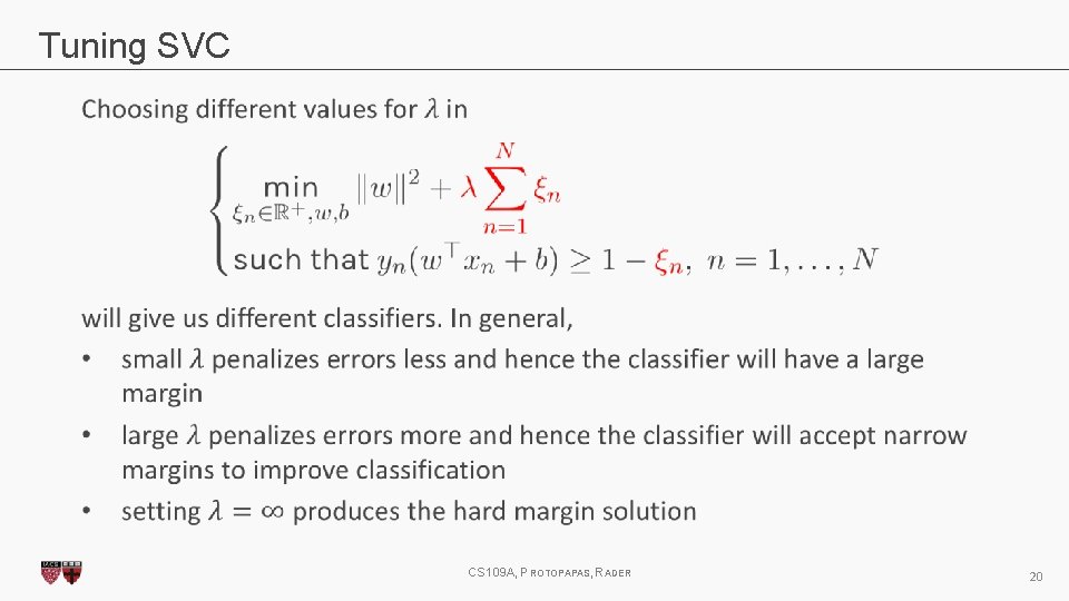
Tuning SVC CS 109 A, PROTOPAPAS, RADER 20

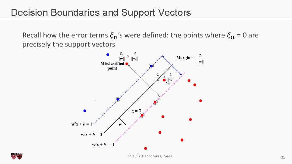
Decision Boundaries and Support Vectors CS 109 A, PROTOPAPAS, RADER 21

Decision Boundaries and Support Vectors Thus to re-construct the decision boundary, only the support vectors are needed! CS 109 A, PROTOPAPAS, RADER 22

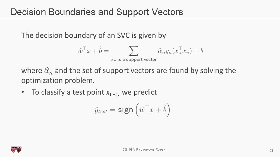
Decision Boundaries and Support Vectors CS 109 A, PROTOPAPAS, RADER 23

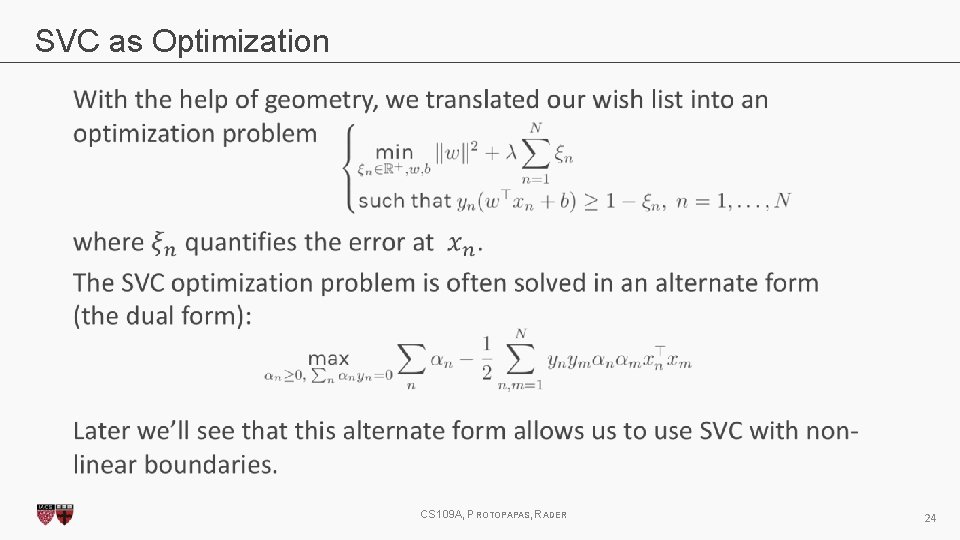
SVC as Optimization CS 109 A, PROTOPAPAS, RADER 24

Extension to Non-linear Boundaries CS 109 A, PROTOPAPAS, RADER 25

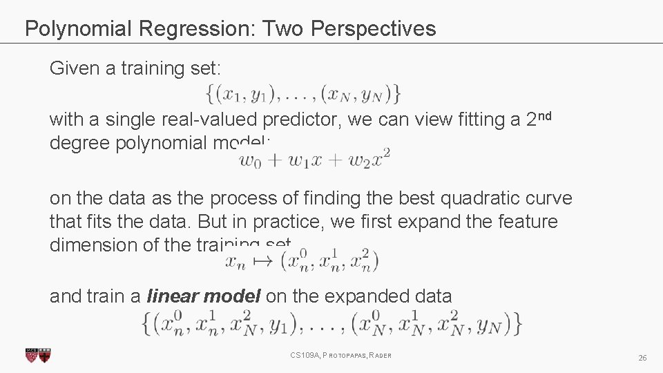
Polynomial Regression: Two Perspectives Given a training set: with a single real-valued predictor, we can view fitting a 2 nd degree polynomial model: on the data as the process of finding the best quadratic curve that fits the data. But in practice, we first expand the feature dimension of the training set and train a linear model on the expanded data CS 109 A, PROTOPAPAS, RADER 26

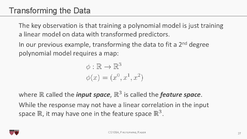
Transforming the Data CS 109 A, PROTOPAPAS, RADER 27

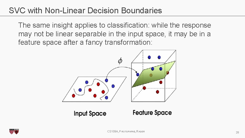
SVC with Non-Linear Decision Boundaries The same insight applies to classification: while the response may not be linear separable in the input space, it may be in a feature space after a fancy transformation: CS 109 A, PROTOPAPAS, RADER 28

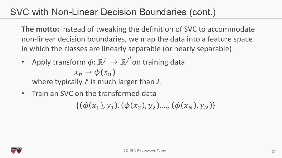
SVC with Non-Linear Decision Boundaries (cont. ) CS 109 A, PROTOPAPAS, RADER 29

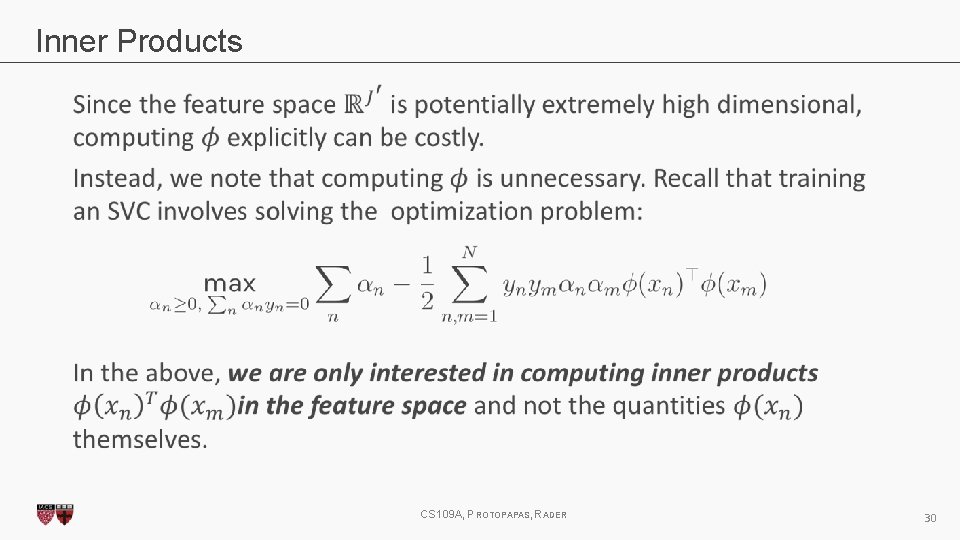
Inner Products CS 109 A, PROTOPAPAS, RADER 30

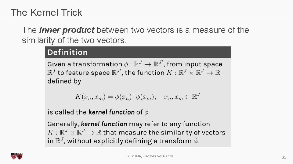
The Kernel Trick The inner product between two vectors is a measure of the similarity of the two vectors. CS 109 A, PROTOPAPAS, RADER 31

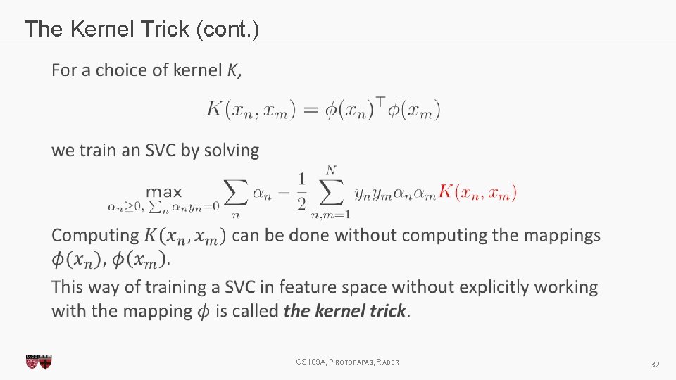
The Kernel Trick (cont. ) CS 109 A, PROTOPAPAS, RADER 32

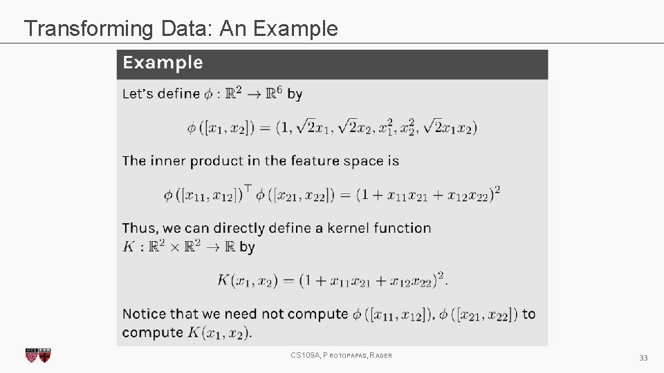
Transforming Data: An Example CS 109 A, PROTOPAPAS, RADER 33

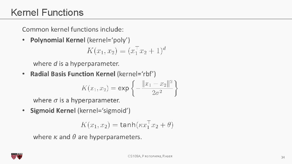
Kernel Functions CS 109 A, PROTOPAPAS, RADER 34

Happy Thanksgiving! CS 109 A, PROTOPAPAS, RADER 35