LECTURE 2 UTILITY AND RISK AVERSION Asset Pricing

LECTURE 2 : UTILITY AND RISK AVERSION (Asset Pricing and Portfolio Theory)

Contents Introduction to utility theory n Relative and absolute risk aversion n Different forms of utility functions n Empirical evidence n How useful are the general findings ? n – Equity premium puzzle – Risk free rate puzzle

Introduction Many different investment opportunities with different risk – return characteristics n General assumption : ‘Like returns, dislike risk’ n Preferences of investors (like more to less) n

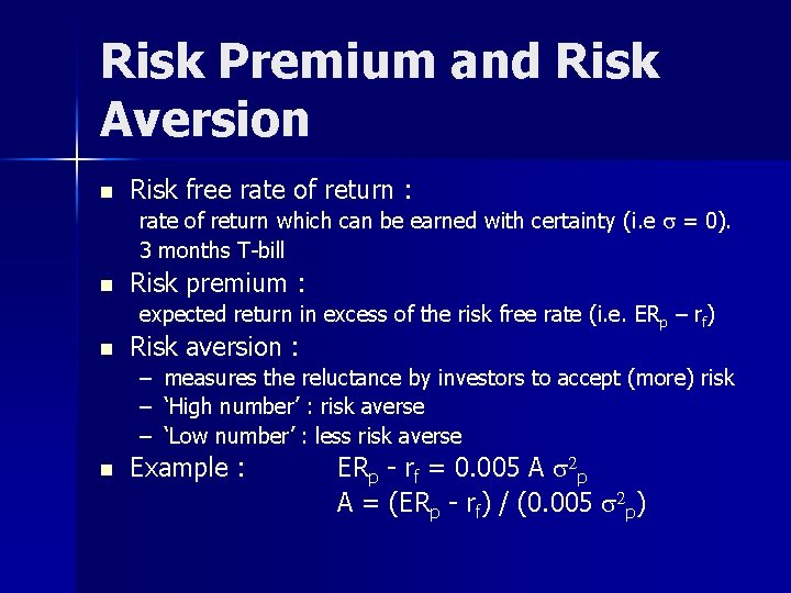
Risk Premium and Risk Aversion n Risk free rate of return : rate of return which can be earned with certainty (i. e s = 0). 3 months T-bill n Risk premium : expected return in excess of the risk free rate (i. e. ERp – rf) n Risk aversion : – – – n measures the reluctance by investors to accept (more) risk ‘High number’ : risk averse ‘Low number’ : less risk averse Example : ERp - rf = 0. 005 A s 2 p A = (ERp - rf) / (0. 005 s 2 p)

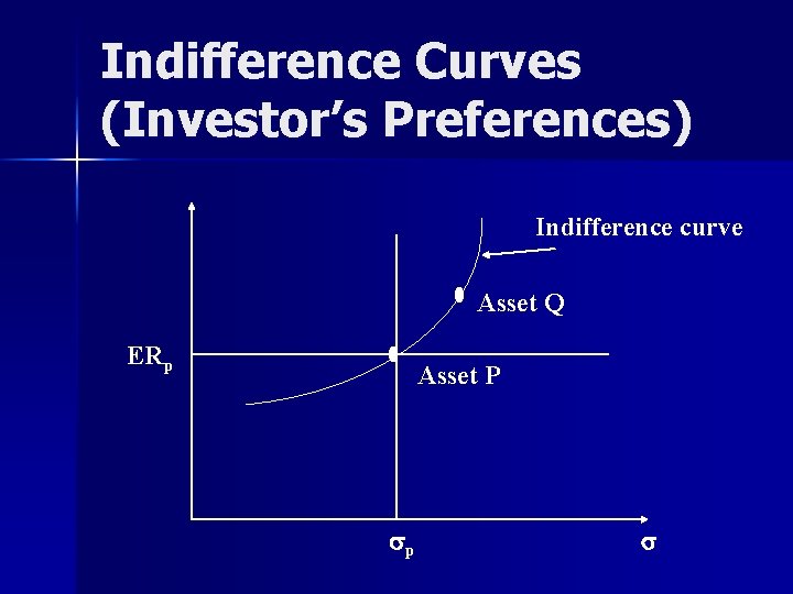
Indifference Curves (Investor’s Preferences) Indifference curve Asset Q ERp Asset P sp s

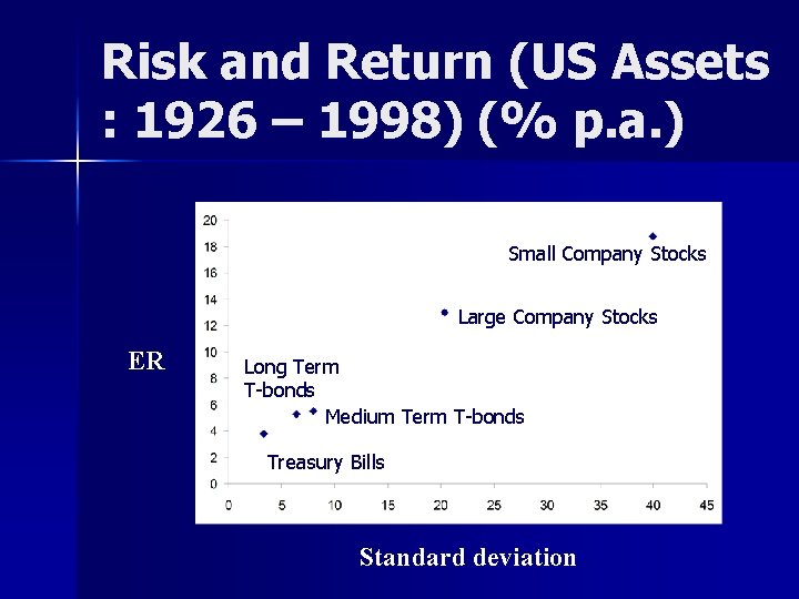
Risk and Return (US Assets : 1926 – 1998) (% p. a. ) Small Company Stocks Large Company Stocks ER Long Term T-bonds Medium Term T-bonds Treasury Bills Standard deviation

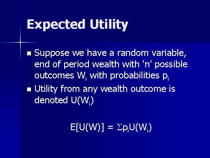
Expected Utility Suppose we have a random variable, end of period wealth with ‘n’ possible outcomes Wi with probabilities pi n Utility from any wealth outcome is denoted U(Wi) n E[U(W)] = Spi. U(Wi)

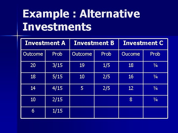
Example : Alternative Investments Investment A Investment B Investment C Outcome Prob Oucome Prob 20 3/15 19 1/5 18 ¼ 18 5/15 10 2/5 16 ¼ 14 4/15 5 2/5 12 ¼ 10 2/15 8 ¼ 6 1/15

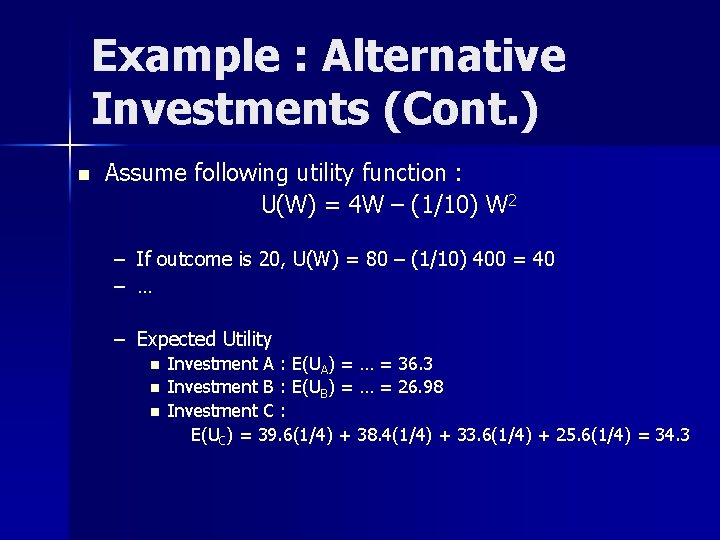
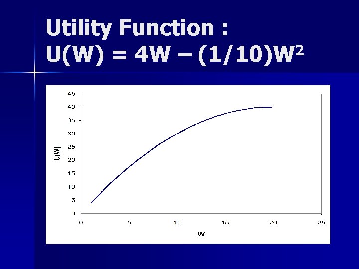
Example : Alternative Investments (Cont. ) n Assume following utility function : U(W) = 4 W – (1/10) W 2 – If outcome is 20, U(W) = 80 – (1/10) 400 = 40 – … – Expected Utility n n n Investment A : E(UA) = … = 36. 3 Investment B : E(UB) = … = 26. 98 Investment C : E(UC) = 39. 6(1/4) + 38. 4(1/4) + 33. 6(1/4) + 25. 6(1/4) = 34. 3

Utility Function : 2 U(W) = 4 W – (1/10)W

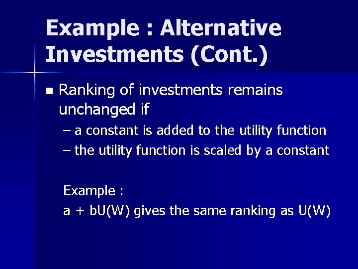
Example : Alternative Investments (Cont. ) n Ranking of investments remains unchanged if – a constant is added to the utility function – the utility function is scaled by a constant Example : a + b. U(W) gives the same ranking as U(W)

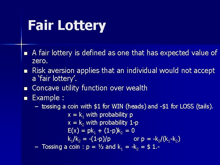
Fair Lottery n n A fair lottery is defined as one that has expected value of zero. Risk aversion applies that an individual would not accept a ‘fair lottery’. Concave utility function over wealth Example : – tossing a coin with $1 for WIN (heads) and -$1 for LOSS (tails). x = k 1 with probability p x = k 2 with probability 1 -p E(x) = pk 1 + (1 -p)k 2 = 0 k 1/k 2 = -(1 -p)/p or p = -k 2/(k 1 -k 2) – Tossing a coin : p = ½ and k 1 = -k 2 = $ 1. -

Utility : The Basics

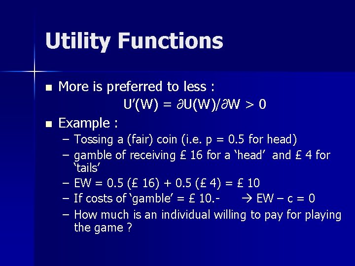
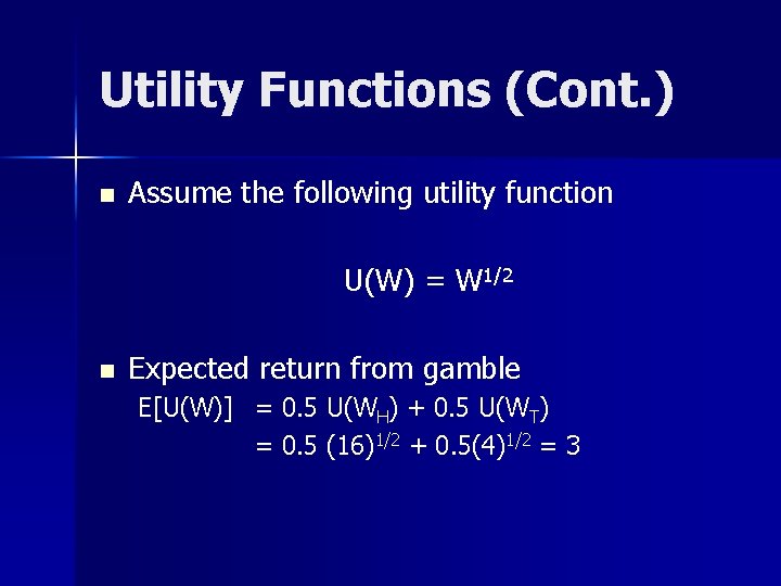
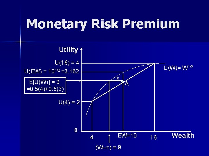
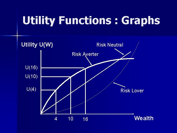
Utility Functions n n More is preferred to less : U’(W) = ∂U(W)/∂W > 0 Example : – Tossing a (fair) coin (i. e. p = 0. 5 for head) – gamble of receiving £ 16 for a ‘head’ and £ 4 for ‘tails’ – EW = 0. 5 (£ 16) + 0. 5 (£ 4) = £ 10 – If costs of ‘gamble’ = £ 10. EW – c = 0 – How much is an individual willing to pay for playing the game ?

Utility Functions (Cont. ) n Assume the following utility function U(W) = W 1/2 n Expected return from gamble E[U(W)] = 0. 5 U(WH) + 0. 5 U(WT) = 0. 5 (16)1/2 + 0. 5(4)1/2 = 3

Monetary Risk Premium Utility U(16) = 4 U(EW) = 101/2 =3. 162 U(W)= W 1/2 p E[U(W)] = 3 =0. 5(4)+0. 5(2) A U(4) = 2 0 4 EW=10 (W–p) = 9 16 Wealth

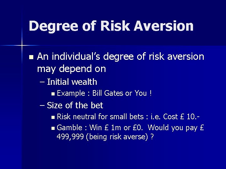
Degree of Risk Aversion n An individual’s degree of risk aversion may depend on – Initial wealth n Example : Bill Gates or You ! – Size of the bet n Risk neutral for small bets : i. e. Cost £ 10. n Gamble : Win £ 1 m or £ 0. Would you pay £ 499, 999 (being risk averse) ?

Absolute and Relative Risk Aversion

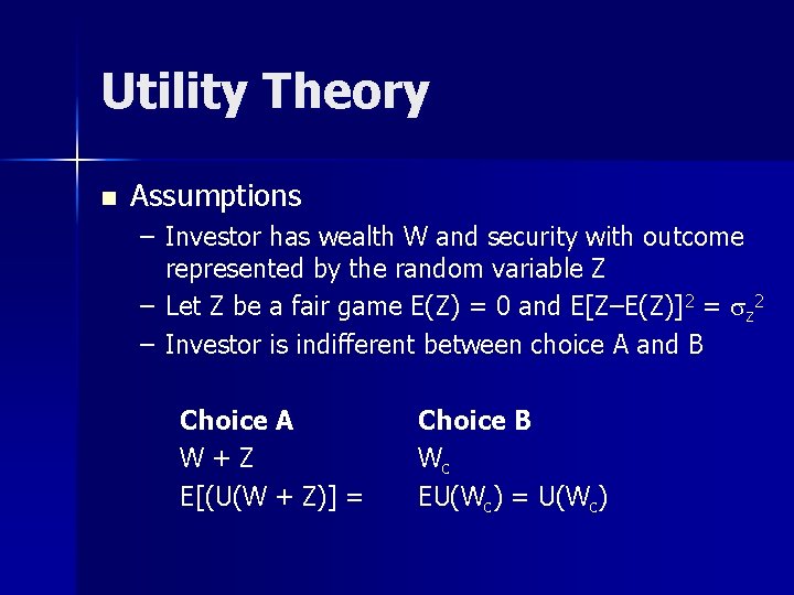
Utility Theory n Assumptions – Investor has wealth W and security with outcome represented by the random variable Z – Let Z be a fair game E(Z) = 0 and E[Z–E(Z)]2 = sz 2 – Investor is indifferent between choice A and B Choice A W+Z E[(U(W + Z)] = Choice B Wc EU(Wc) = U(Wc)

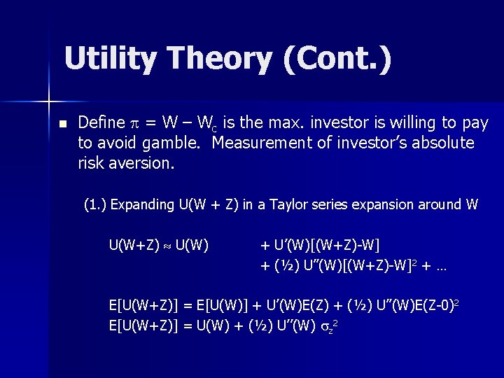
Utility Theory (Cont. ) n Define p = W – Wc is the max. investor is willing to pay to avoid gamble. Measurement of investor’s absolute risk aversion. (1. ) Expanding U(W + Z) in a Taylor series expansion around W U(W+Z) U(W) + U’(W)[(W+Z)-W] + (½) U’’(W)[(W+Z)-W]2 + … E[U(W+Z)] = E[U(W)] + U’(W)E(Z) + (½) U’’(W)E(Z-0) 2 E[U(W+Z)] = U(W) + (½) U’’(W) sz 2

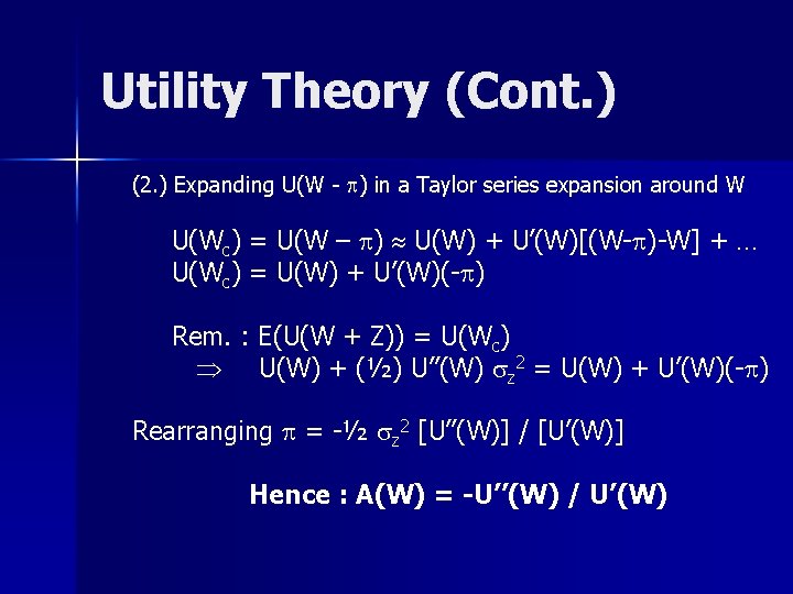
Utility Theory (Cont. ) (2. ) Expanding U(W - p) in a Taylor series expansion around W U(Wc) = U(W – p) U(W) + U’(W)[(W-p)-W] + … U(Wc) = U(W) + U’(W)(-p) Rem. : E(U(W + Z)) = U(Wc) U(W) + (½) U’’(W) sz 2 = U(W) + U’(W)(-p) Rearranging p = -½ sz 2 [U’’(W)] / [U’(W)] Hence : A(W) = -U’’(W) / U’(W)

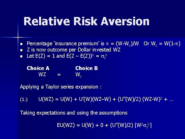
Relative Risk Aversion n Percentage ‘insurance premium’ is p = (W-Wc)/W Or Wc = W(1 -p) Z is now outcome per Dollar invested WZ Let E(Z) = 1 and E(Z – E(Z))2 = sz 2 Choice A WZ = Choice B Wc Applying a Taylor series expansion : (1. ) U(WZ) = U(W) + U’(W)(WZ–W) + (U’’(W)/2) (WZ-W) 2 + … Taking expectations and using the assumptions EU(WZ) = U(W) + 0 + (U’’(W)/2) [W 2 sz 2]

Relative Risk Aversion (Cont. ) (2. ) U(Wc) = U[W(1 – p)] = U(W) + U’(W)[W(1 – p) – W] + … U(Wc) = U(W) + U’(W) (-p. W) U(W) + ½ U’’(W) sz 2 W 2 = U(W) – p. WU’(W) p = -(sz 2 /2) [WU’’(W) / U’(W)] Hence : R(W) = -WU’’(W) / U’(W)

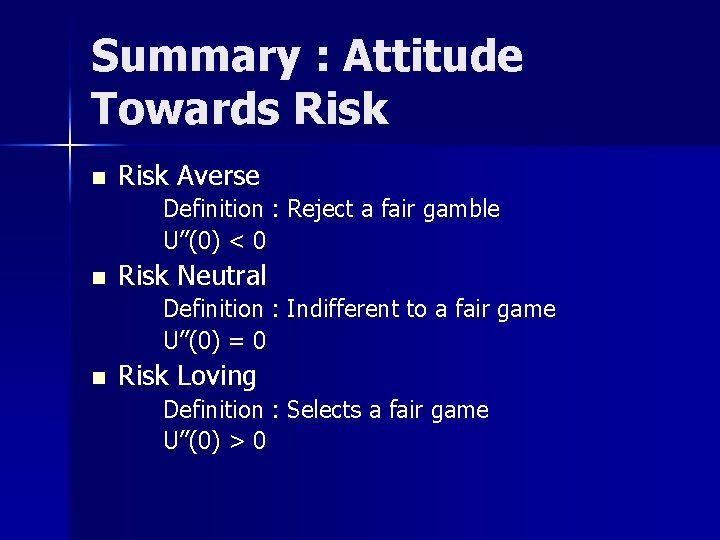
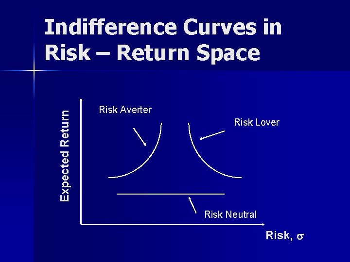
Summary : Attitude Towards Risk n Risk Averse Definition : Reject a fair gamble U’’(0) < 0 n Risk Neutral Definition : Indifferent to a fair game U’’(0) = 0 n Risk Loving Definition : Selects a fair game U’’(0) > 0

Utility Functions : Graphs Utility U(W) Risk Neutral Risk Averter U(16) U(10) U(4) Risk Lover 4 10 16 Wealth

Expected Return Indifference Curves in Risk – Return Space Risk Averter Risk Lover Risk Neutral Risk, s

Examples of Utility Functions

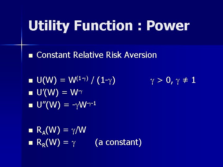
Utility Function : Power n n n Constant Relative Risk Aversion U(W) = W(1 -g) / (1 -g) U’(W) = W-g U’’(W) = -g. W-g-1 RA(W) = g/W RR(W) = g (a constant) g > 0, g ≠ 1

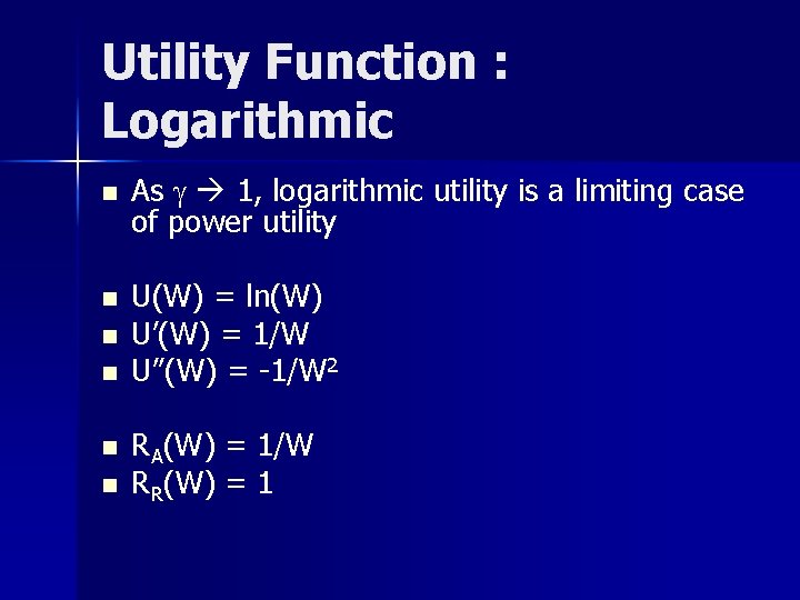
Utility Function : Logarithmic n n n As g 1, logarithmic utility is a limiting case of power utility U(W) = ln(W) U’(W) = 1/W U’’(W) = -1/W 2 RA(W) = 1/W RR(W) = 1

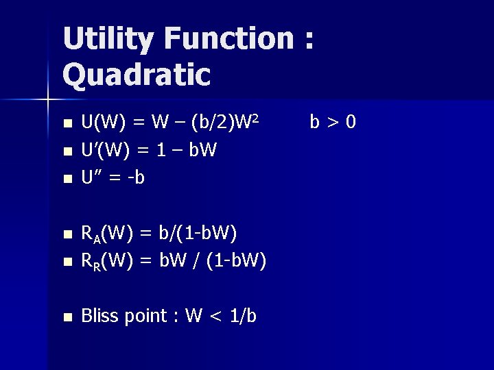
Utility Function : Quadratic n n n U(W) = W – (b/2)W 2 U’(W) = 1 – b. W U’’ = -b n RA(W) = b/(1 -b. W) RR(W) = b. W / (1 -b. W) n Bliss point : W < 1/b n b>0

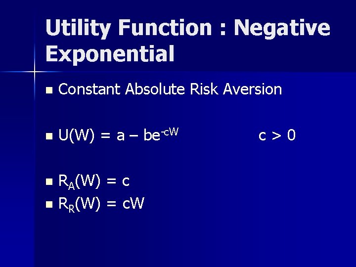
Utility Function : Negative Exponential n Constant Absolute Risk Aversion n U(W) = a – be-c. W RA(W) = c n RR(W) = c. W n c>0

Empirical Evidence

How does it Work in the ‘Real World’ ? n To investigate whether (specific) utility functions represent behaviour of economic agents : – Experimental evidence from simple choice situations – Survey data on investor’s asset choices

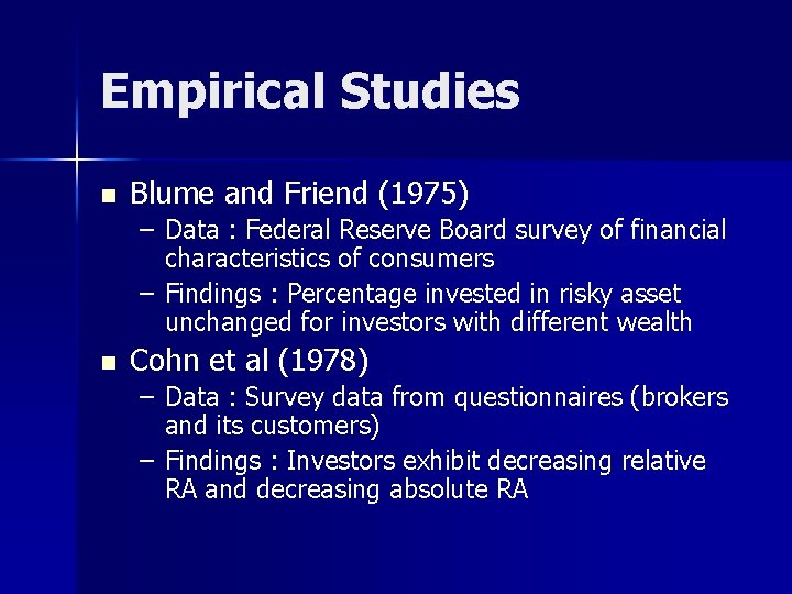
Empirical Studies n Blume and Friend (1975) – Data : Federal Reserve Board survey of financial characteristics of consumers – Findings : Percentage invested in risky asset unchanged for investors with different wealth n Cohn et al (1978) – Data : Survey data from questionnaires (brokers and its customers) – Findings : Investors exhibit decreasing relative RA and decreasing absolute RA

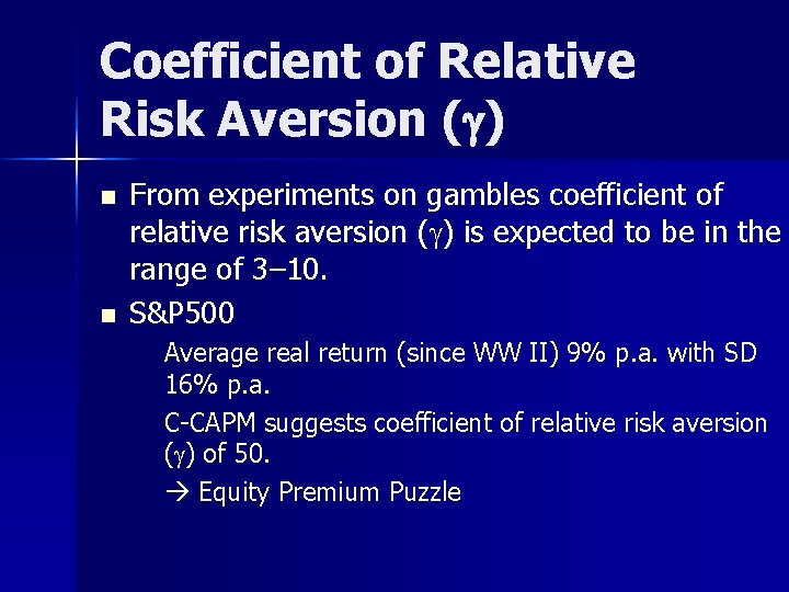
Coefficient of Relative Risk Aversion (g) n n From experiments on gambles coefficient of relative risk aversion (g) is expected to be in the range of 3– 10. S&P 500 Average real return (since WW II) 9% p. a. with SD 16% p. a. C-CAPM suggests coefficient of relative risk aversion (g) of 50. Equity Premium Puzzle

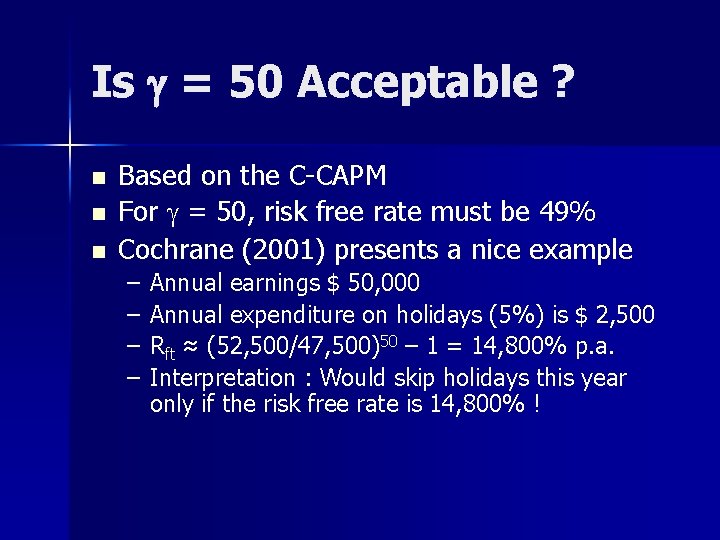
Is g = 50 Acceptable ? n n n Based on the C-CAPM For g = 50, risk free rate must be 49% Cochrane (2001) presents a nice example – – Annual earnings $ 50, 000 Annual expenditure on holidays (5%) is $ 2, 500 Rft ≈ (52, 500/47, 500)50 – 1 = 14, 800% p. a. Interpretation : Would skip holidays this year only if the risk free rate is 14, 800% !

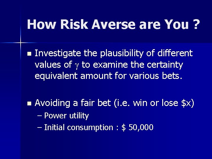
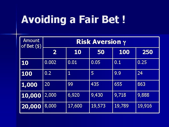
How Risk Averse are You ? n Investigate the plausibility of different values of g to examine the certainty equivalent amount for various bets. n Avoiding a fair bet (i. e. win or lose $x) – Power utility – Initial consumption : $ 50, 000

Avoiding a Fair Bet ! Risk Aversion g Amount of Bet ($) 2 10 50 100 250 10 0. 002 0. 01 0. 05 0. 1 0. 25 100 0. 2 1 5 9. 9 24 1, 000 20 99 435 655 863 10, 000 2, 000 6, 920 9, 430 9, 718 9, 888 20, 000 8, 000 17, 600 19, 573 19, 789 19, 916

Application : Mean Variance Model

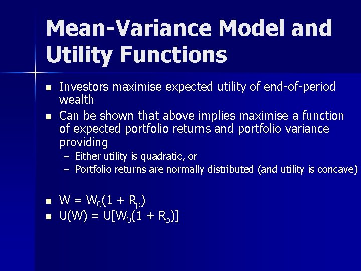
Mean-Variance Model and Utility Functions n n Investors maximise expected utility of end-of-period wealth Can be shown that above implies maximise a function of expected portfolio returns and portfolio variance providing – Either utility is quadratic, or – Portfolio returns are normally distributed (and utility is concave) n n W = W 0(1 + Rp) U(W) = U[W 0(1 + Rp)]

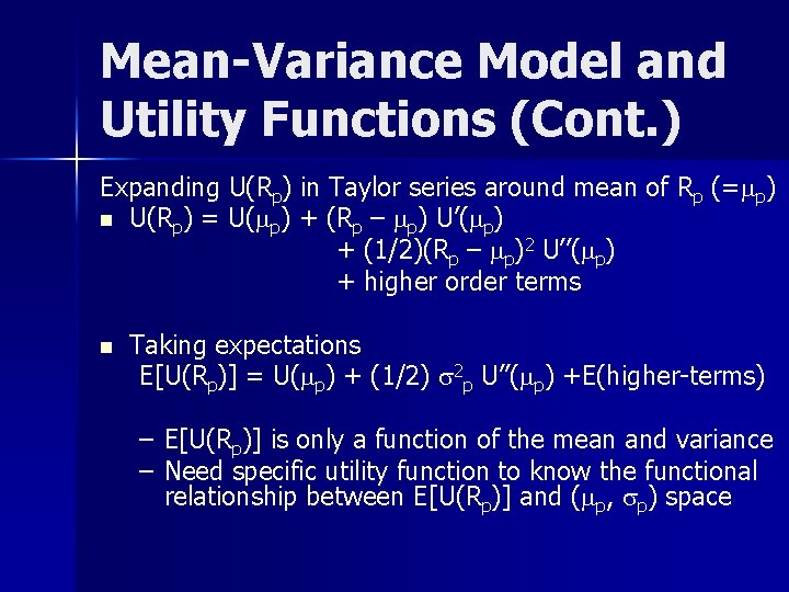
Mean-Variance Model and Utility Functions (Cont. ) Expanding U(Rp) in Taylor series around mean of Rp (=mp) n U(Rp) = U(mp) + (Rp – mp) U’(mp) + (1/2)(Rp – mp)2 U’’(mp) + higher order terms n Taking expectations E[U(Rp)] = U(mp) + (1/2) s 2 p U’’(mp) +E(higher-terms) – E[U(Rp)] is only a function of the mean and variance – Need specific utility function to know the functional relationship between E[U(Rp)] and (mp, sp) space

Summary Utility functions, expected utility n Different measures of risk aversion : absolute, relative n Attitude towards risk, indifference curves n Empirical evidence and an application of utility analysis n

References n Cuthbertson, K. and Nitzsche, D. (2004) ‘Quantitative Financial Economics’, Chapter 1

References n n n Blume, M. and Friend, I. (1975) ‘The Asset Structure of Individual Portfolios and Some Implications for Utility Functions’, Journal of Finance, Vol. 10(2), pp. 585 -603 Cohn, R. , Lewellen, W. , Lease, R. and Schlarbaum, G. (1975) ‘Individual Investor Risk Aversion and Investment Portfolio Composition’, Journal of Finance, Vol. 10(2), pp. 605 -620. Cochrane, J. H. (2001) Asset Pricing, Princeton University Press

END OF LECTURE