Lecture 2 Testing the implications of the DMF

Lecture 2: Testing the implications of the DMF model Birmingham MSc International Macro Autumn 2015 Tony Yates

Recap on DMF model implications • The nominal exchange rate ‘overshoots’ its long run resting level following a change in the money stock. • Money stock changes cause changes in the REAL exchange rate. • Both things may be costly for society. • So, if DMF model is true, implies caution in changing the money stock!

Overview • Just as in lecture 1 – there will be an informal, story telling approach to how econometricians tested the DMF model – And a formal part that you can go through yourself, explored also in the classes. – The analysis is based on Clarida-Gali, which is on the reading list. – It’s a hard paper, and put there for completeness. But at least have a look at the introduction and the conclusions.

Questions we want answers to? • What happens to the nominal exchange rate when the money stock changes? • How much of real exchange rate changes are due to changes in the money stock. • We are going to describe some strategies that DON’T work, explain why they don’t, and then state what econometricians did instead.

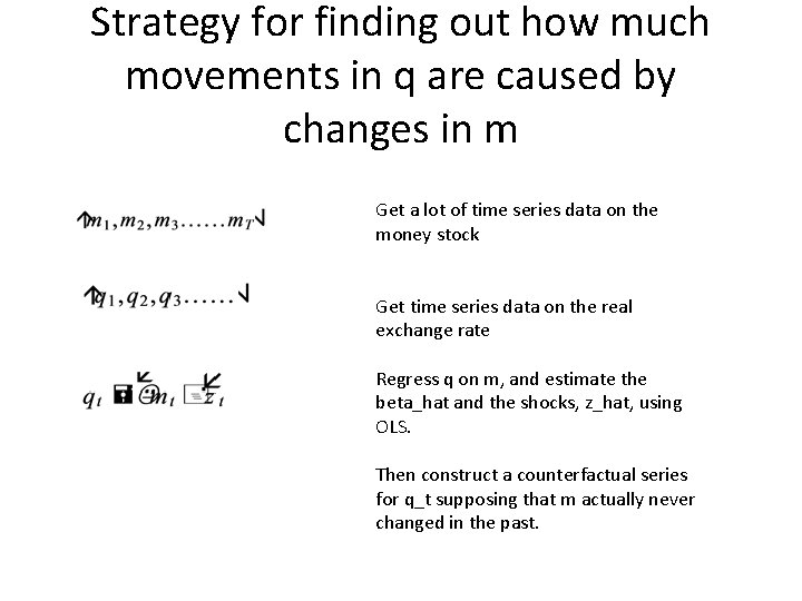
Strategy for finding out how much movements in q are caused by changes in m Get a lot of time series data on the money stock Get time series data on the real exchange rate Regress q on m, and estimate the beta_hat and the shocks, z_hat, using OLS. Then construct a counterfactual series for q_t supposing that m actually never changed in the past.

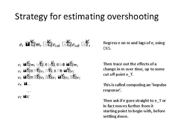
Strategy for estimating overshooting Regress e on m and lags of e, using OLS. Then trace out the effects of a change in m over time, up to some cut off point e_T. This is called computing an ‘impulse response’. Then ask if e goes straight to e_T or in fact moves further from it starting point to begin with, before settling down.

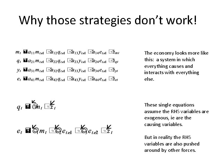
Why those strategies don’t work! The economy looks more like this: a system in which everything causes and interacts with everything else. These single equations assume the RHS variables are exogenous, ie are the causing variables. But in reality the RHS variables are also pushed around by other forces.

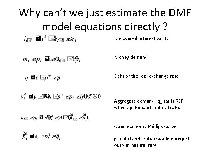
Why can’t we just estimate the DMF model equations directly ? Uncovered interest parity Money demand Defn of the real exchange rate Aggregate demand. q_bar is RER when ag demand=natural rate. Open economy Phillips Curve p_tilda is price that would emerge if output=natural rate.

So why not just estimate the DMF model directly? • Take model equations. Find data for m, q, e, p, p_star, y…. • Estimate phi, delta, etc by OLS, see if phi*delta<1…. . • Real world is more complicated. DMF model is incomplete. • Misses out: govt; technology shocks; demand shocks, labour market…. .

Why we don’t want to estimate the DMF model directly • If we did, our estimates (of the effects of m on q, for example) would only be as good as our assumption that the DMF model was true. • All models are false! So we want a strategy for answering our questions that doesn’t assume too many things we are not sure of. • Estimating a vector autoregression [that system of equations we saw] allows us to do this.

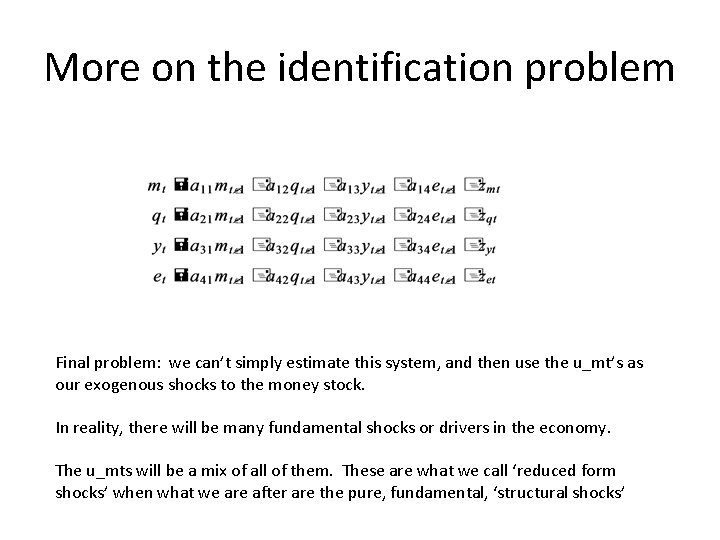
More on the identification problem Final problem: we can’t simply estimate this system, and then use the u_mt’s as our exogenous shocks to the money stock. In reality, there will be many fundamental shocks or drivers in the economy. The u_mts will be a mix of all of them. These are what we call ‘reduced form shocks’ when what we are after are the pure, fundamental, ‘structural shocks’

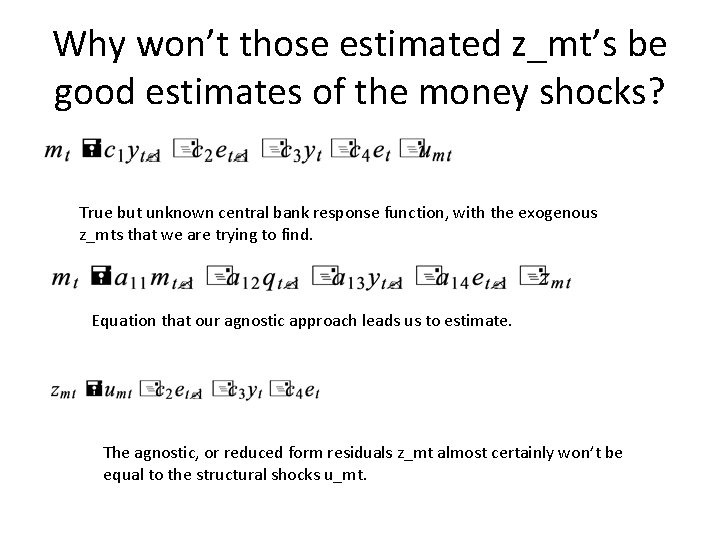
Why won’t those estimated z_mt’s be good estimates of the money shocks? True but unknown central bank response function, with the exogenous z_mts that we are trying to find. Equation that our agnostic approach leads us to estimate. The agnostic, or reduced form residuals z_mt almost certainly won’t be equal to the structural shocks u_mt.

So what did Clarida-Gali do instead? • Estimate a vector autoregression. • Use some elements of DMF theory which is also common to other theories and not so controversial. • Notion that monetary shocks should not affect real things [q, y] in the long run, but will in the short run. • And real things don’t affect nominal things [like the money stock] in the long run.

Clarida-Gali • Those assumptions allowed CG to disentangle the exogenous money shocks from the reduced form shock ‘mixture’… • …and measure the response of the exchange rate. • They found overshooting in the impulse response of e to the money shocks. • With the structural money shocks, can also quantify the contribution of them to volatility in the real exchange rate. • This was sizeable!

Formal analysis of Long Run restrictions • Hard! • Some analysis of the matrix algebra of vector autoregressions. • Covered in detail in the lecture notes and the problem sets. • But let’s have a go. Either today or at the end of the course, when your algebra muscles are hardened.

Concepts used along the way • • Inverse of a square matrix A^-1, like dividing by a scalar. Matrix multiplication. Transpose of a matrix A’ [mirror image about diagonal] Variance, covariance, expected value. [ie E[(x-x_bar)(yy_bar)] Ordinary Least Squares [OLS] estimates [(x’x)^-1*(x’y)] Impulse response. ‘the impact of a shock traced out through the model over time’. Exogeneity, endogeneity. See my lecture notes on time series from last year at Bristol.

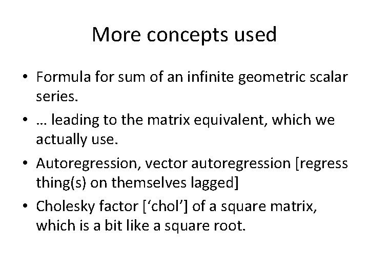
More concepts used • Formula for sum of an infinite geometric scalar series. • … leading to the matrix equivalent, which we actually use. • Autoregression, vector autoregression [regress thing(s) on themselves lagged] • Cholesky factor [‘chol’] of a square matrix, which is a bit like a square root.

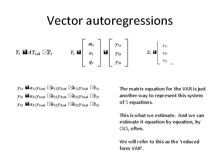
Vector autoregressions The matrix equation for the VAR is just another way to represent this system of 3 equations. This is what we estimate. And we can estimate it equation by equation, by OLS, often. We will refer to this as the ‘reduced form VAR’.

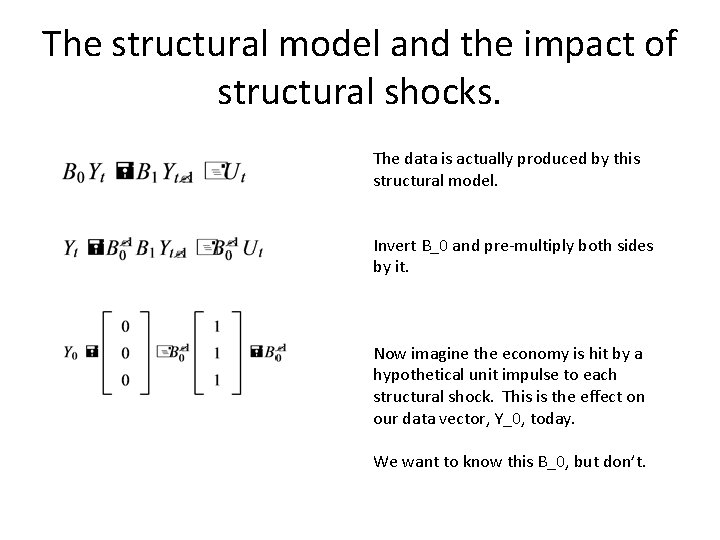
The structural model and the impact of structural shocks. The data is actually produced by this structural model. Invert B_0 and pre-multiply both sides by it. Now imagine the economy is hit by a hypothetical unit impulse to each structural shock. This is the effect on our data vector, Y_0, today. We want to know this B_0, but don’t.

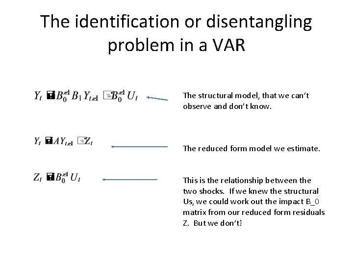
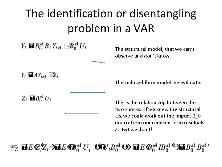
The identification or disentangling problem in a VAR The structural model, that we can’t observe and don’t know. The reduced form model we estimate. This is the relationship between the two shocks. If we knew the structural Us, we could work out the impact B_0 matrix from our reduced form residuals Z. But we don’t!

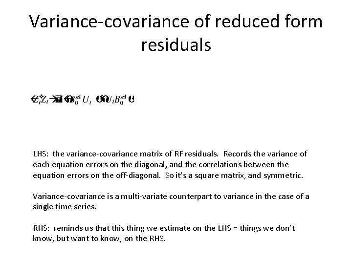
Variance-covariance of reduced form residuals LHS: the variance-covariance matrix of RF residuals. Records the variance of each equation errors on the diagonal, and the correlations between the equation errors on the off-diagonal. So it’s a square matrix, and symmetric. Variance-covariance is a multi-variate counterpart to variance in the case of a single time series. RHS: reminds us that this thing we estimate on the LHS = things we don’t know, but want to know, on the RHS.

Variance-covariance in univariate case This is how we would compute the variance of residuals in a 1 time-series regression…… OLS formula Residual computed from fitted value

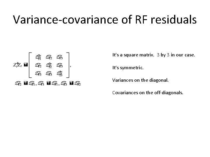
Variance-covariance of RF residuals It’s a square matrix. 3 by 3 in our case. It’s symmetric. Variances on the diagonal. Covariances on the off-diagonals.

The identification or disentangling problem in a VAR The structural model, that we can’t observe and don’t know. The reduced form model we estimate. This is the relationship between the two shocks. If we knew the structural Us, we could work out the impact B_0 matrix from our reduced form residuals Z. But we don’t!

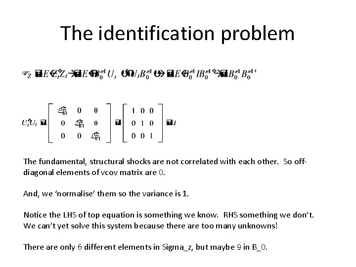
The identification problem The fundamental, structural shocks are not correlated with each other. So offdiagonal elements of vcov matrix are 0. And, we ‘normalise’ them so the variance is 1. Notice the LHS of top equation is something we know. RHS something we don’t. We can’t yet solve this system because there are too many unknowns! There are only 6 different elements in Sigma_z, but maybe 9 in B_0.

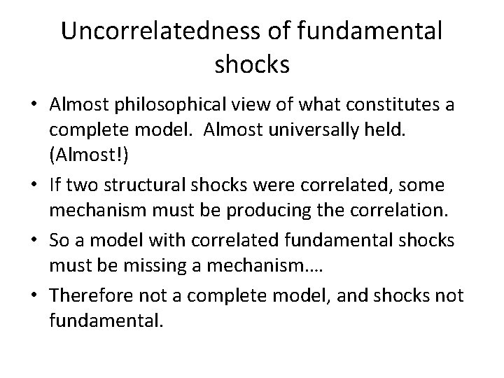
Uncorrelatedness of fundamental shocks • Almost philosophical view of what constitutes a complete model. Almost universally held. (Almost!) • If two structural shocks were correlated, some mechanism must be producing the correlation. • So a model with correlated fundamental shocks must be missing a mechanism…. • Therefore not a complete model, and shocks not fundamental.

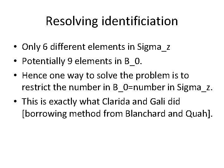
Resolving identificiation • Only 6 different elements in Sigma_z • Potentially 9 elements in B_0. • Hence one way to solve the problem is to restrict the number in B_0=number in Sigma_z. • This is exactly what Clarida and Gali did [borrowing method from Blanchard and Quah].

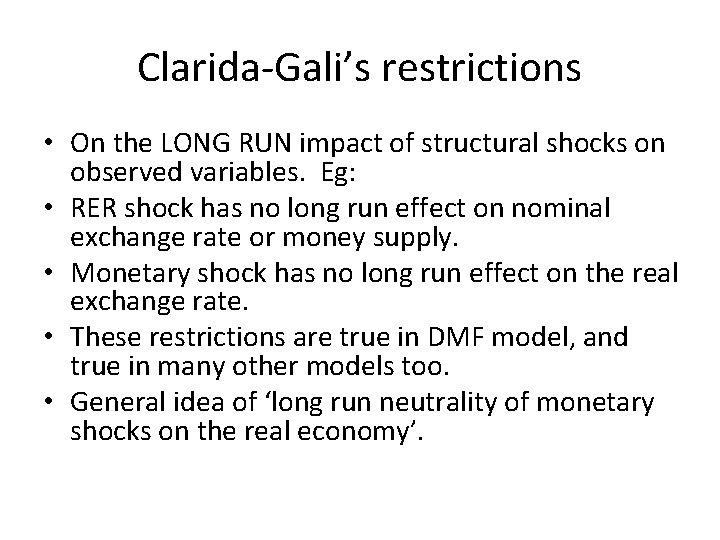
Clarida-Gali’s restrictions • On the LONG RUN impact of structural shocks on observed variables. Eg: • RER shock has no long run effect on nominal exchange rate or money supply. • Monetary shock has no long run effect on the real exchange rate. • These restrictions are true in DMF model, and true in many other models too. • General idea of ‘long run neutrality of monetary shocks on the real economy’.

Formal steps yet to accomplish • See how restrictions on the long run impact actually translate into restrictions on B_0 which measures the short run impact. • See exactly how we would compute things we need to know, like the impact of our variables to an identified shock…. • These steps are tricky.

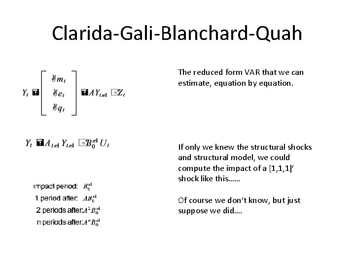
Clarida-Gali-Blanchard-Quah The reduced form VAR that we can estimate, equation by equation. If only we knew the structural shocks and structural model, we could compute the impact of a [1, 1, 1]’ shock like this…… Of course we don’t know, but just suppose we did….

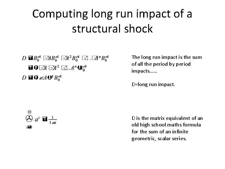
Computing long run impact of a structural shock The long run impact is the sum of all the period by period impacts…… D=long run impact. D is the matrix equivalent of an old high school maths formula for the sum of an infinite geometric, scalar series.

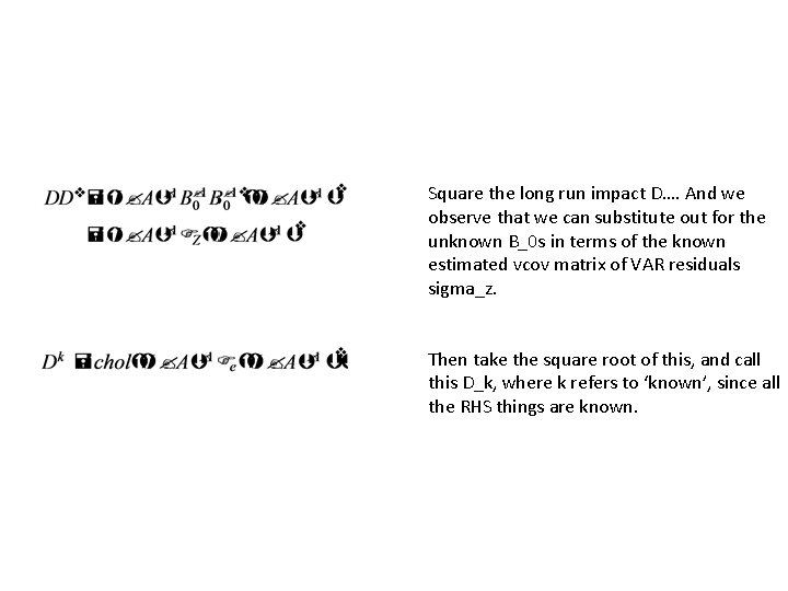
Square the long run impact D…. And we observe that we can substitute out for the unknown B_0 s in terms of the known estimated vcov matrix of VAR residuals sigma_z. Then take the square root of this, and call this D_k, where k refers to ‘known’, since all the RHS things are known.

…finally we find the elusive B_0 Recall the version of the equation for D in terms of D_u, or [in terms of unknowns] Rearrange it so that it’s an equation for the unknown B_0 And then remember we can substitute in for D_u our expression for D_k, which was in terms of knowns. This means we have found the elusive B_0! At this point, you should be jumping with excitement… But in case you forgot what we were doing….

The identification or disentangling problem in a VAR The structural model, that we can’t observe and don’t know. The reduced form model we estimate. This is the relationship between the two shocks. If we knew the structural Us, we could work out the impact B_0 matrix from our reduced form residuals Z. But we don’t!

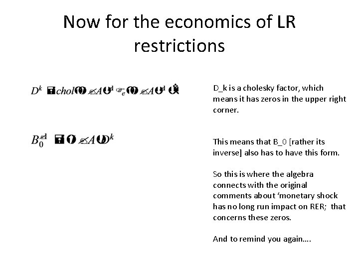
Now for the economics of LR restrictions D_k is a cholesky factor, which means it has zeros in the upper right corner. This means that B_0 [rather its inverse] also has to have this form. So this is where the algebra connects with the original comments about ‘monetary shock has no long run impact on RER; that concerns these zeros. And to remind you again….

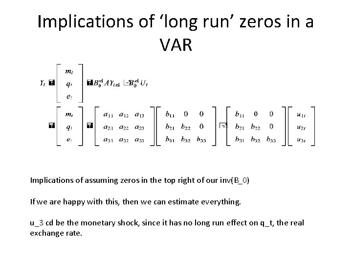
Implications of ‘long run’ zeros in a VAR Implications of assuming zeros in the top right of our inv(B_0) If we are happy with this, then we can estimate everything. u_3 cd be the monetary shock, since it has no long run effect on q_t, the real exchange rate.

Problems with Long Run Restrictions • Don’t work well in small samples [where the long run isn’t well estimated]. • Answers only as good as the restrictions themselves. Finding uncontroversial ones sometimes difficult. • As with any VAR analysis, if you miss out an important variable, your rf shocks won’t ‘span’ the structural shocks. • But putting lots of variables in means imprecise estimates of the A coefficients • Which multiply up in long run analysis.