Lecture 2 Stephen G Hall Time Series Forecasting

Lecture 2 Stephen G Hall Time Series Forecasting

Introduction • These are a body of techniques which rely primarily on the statistical properties of the data, either in isolated single series or in groups of series, and do not exploit our understanding of the working of the economy at all.

• The objective is not to build models which are a good representation of the economy with all its complex interconnections, but rather to build simple models which capture the time series behaviour of the data and may be used to provide an adequate basis forecasting alone.

• See `Applied Economic Forecasting Techniques' ed S G Hall, Simon and Schuster, 1994.

Some basic concepts • Two basic types of time series models exist, • these are autoregressive and moving average models.

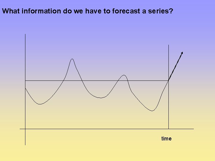
What information do we have to forecast a series? time

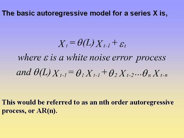
The basic autoregressive model for a series X is, This would be referred to as an nth order autoregressive process, or AR(n).

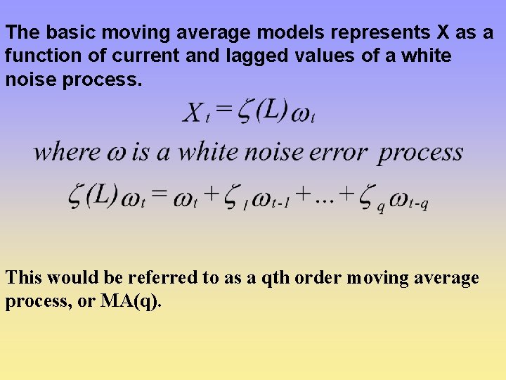
The basic moving average models represents X as a function of current and lagged values of a white noise process. This would be referred to as a qth order moving average process, or MA(q).

ARMA models • A mixture of these two types of model would be referred to as an autoregressive moving average model (ARMA)n, q, where n is the order of the autoregressive part and q is the order of the moving average term.

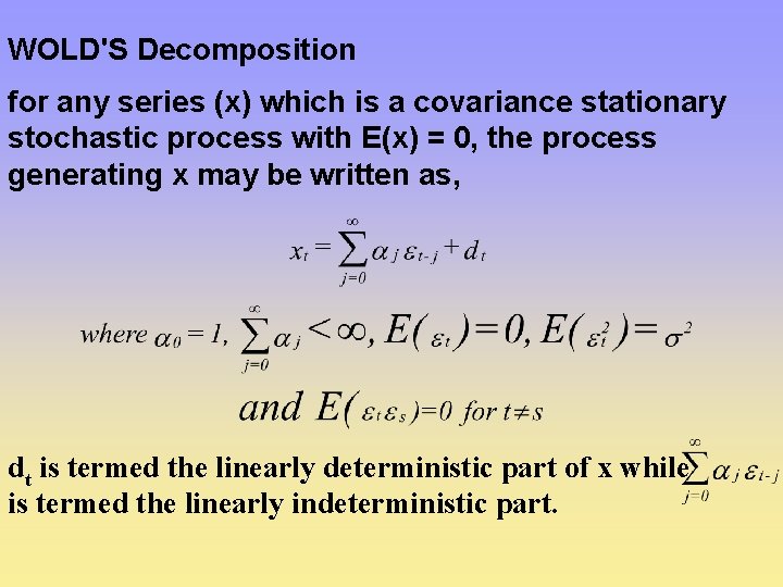
WOLD'S Decomposition for any series (x) which is a covariance stationary stochastic process with E(x) = 0, the process generating x may be written as, dt is termed the linearly deterministic part of x while is termed the linearly indeterministic part.

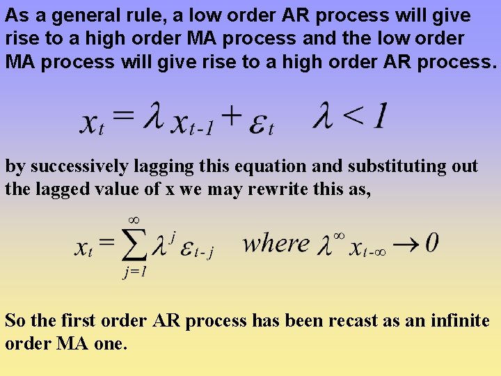
As a general rule, a low order AR process will give rise to a high order MA process and the low order MA process will give rise to a high order AR process. by successively lagging this equation and substituting out the lagged value of x we may rewrite this as, So the first order AR process has been recast as an infinite order MA one.

The Correlogram and partial autocorellation function • Two important tools for diagnosing the time series properties of a series

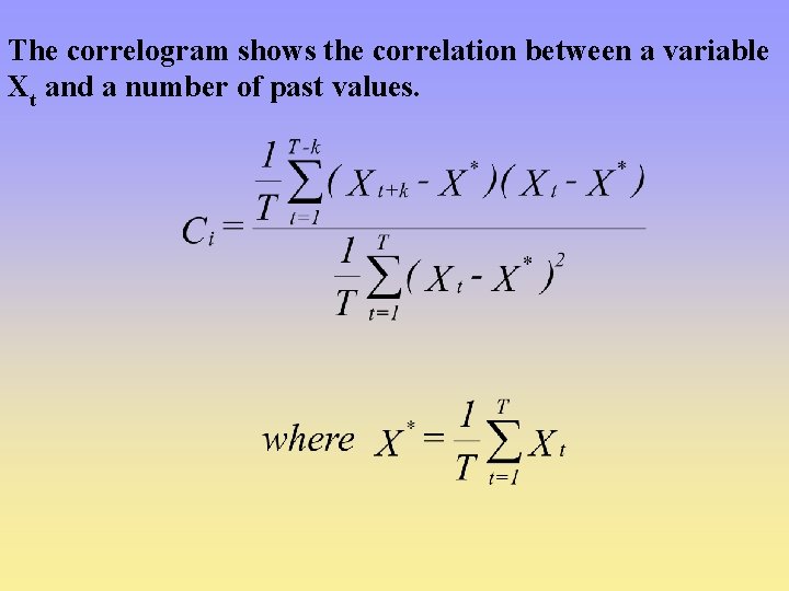
The correlogram shows the correlation between a variable Xt and a number of past values.

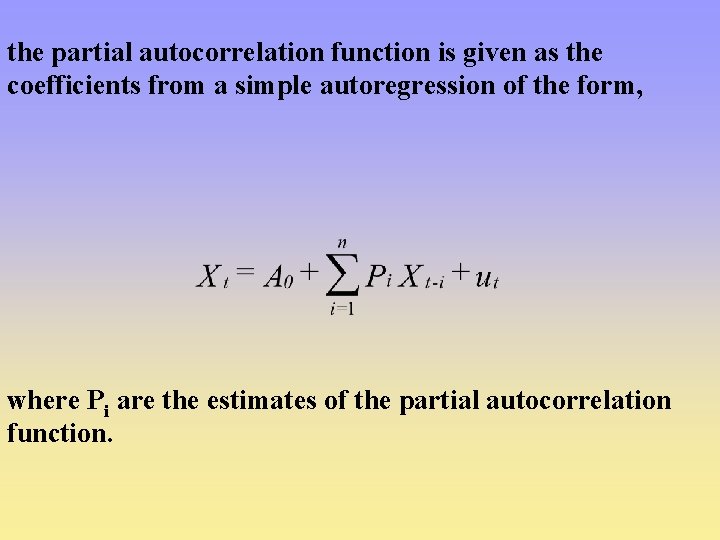
the partial autocorrelation function is given as the coefficients from a simple autoregression of the form, where Pi are the estimates of the partial autocorrelation function.

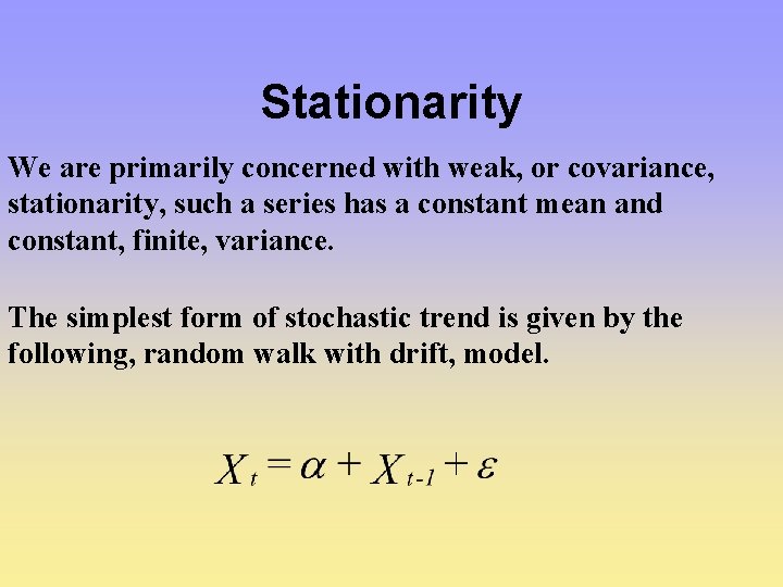
Stationarity We are primarily concerned with weak, or covariance, stationarity, such a series has a constant mean and constant, finite, variance. The simplest form of stochastic trend is given by the following, random walk with drift, model.

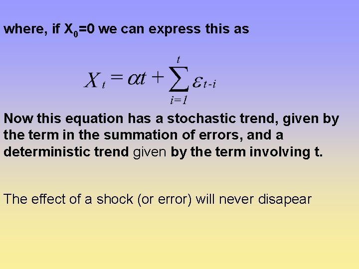
where, if X 0=0 we can express this as Now this equation has a stochastic trend, given by the term in the summation of errors, and a deterministic trend given by the term involving t. The effect of a shock (or error) will never disapear

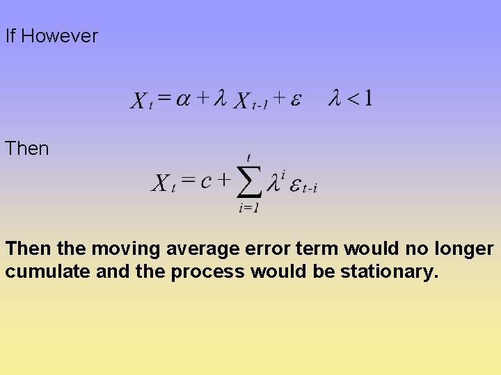
If However Then the moving average error term would no longer cumulate and the process would be stationary.

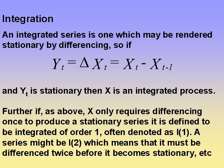
Integration An integrated series is one which may be rendered stationary by differencing, so if and Yt is stationary then X is an integrated process. Further if, as above, X only requires differencing once to produce a stationary series it is defined to be integrated of order 1, often denoted as I(1). A series might be I(2) which means that it must be differenced twice before it becomes stationary, etc

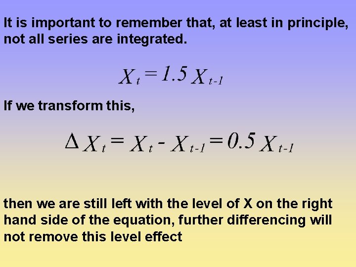
It is important to remember that, at least in principle, not all series are integrated. If we transform this, then we are still left with the level of X on the right hand side of the equation, further differencing will not remove this level effect

`Ad Hoc' forecasting procedures • a broadly sensible approach to forecasting but they are not the result of a particular economic or statistical view about the way the data was generated.

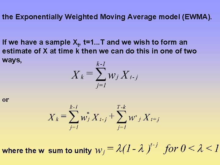
the Exponentially Weighted Moving Average model (EWMA). If we have a sample Xt, t=1. . . T and we wish to form an estimate of X at time k then we can do this in one of two ways, or where the w sum to unity

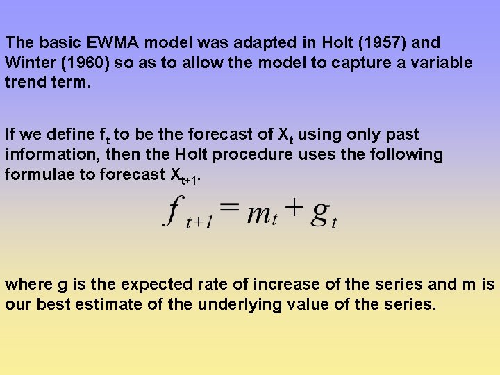
The basic EWMA model was adapted in Holt (1957) and Winter (1960) so as to allow the model to capture a variable trend term. If we define ft to be the forecast of Xt using only past information, then the Holt procedure uses the following formulae to forecast Xt+1. where g is the expected rate of increase of the series and m is our best estimate of the underlying value of the series.

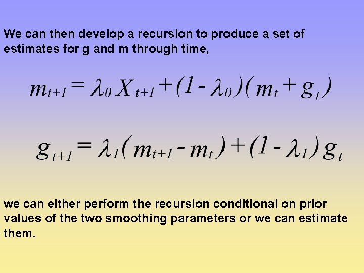
We can then develop a recursion to produce a set of estimates for g and m through time, we can either perform the recursion conditional on prior values of the two smoothing parameters or we can estimate them.

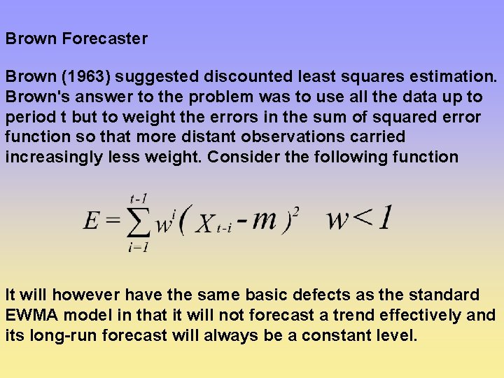
Brown Forecaster Brown (1963) suggested discounted least squares estimation. Brown's answer to the problem was to use all the data up to period t but to weight the errors in the sum of squared error function so that more distant observations carried increasingly less weight. Consider the following function It will however have the same basic defects as the standard EWMA model in that it will not forecast a trend effectively and its long-run forecast will always be a constant level.

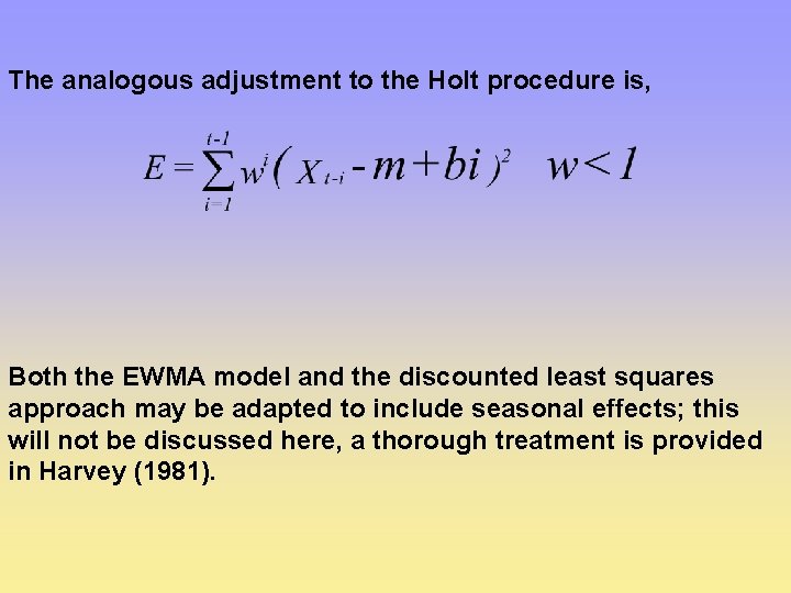
The analogous adjustment to the Holt procedure is, Both the EWMA model and the discounted least squares approach may be adapted to include seasonal effects; this will not be discussed here, a thorough treatment is provided in Harvey (1981).

The Box-Jenkins approach • Box and Jenkins (1976) proposed a modelling strategy for pure time series forecasting • The Box-Jenkins procedure may be seen as one of the early attempts to confront the problem of non-stationary data. • The Box Jenkins modelling procedure consists of three stages; identification, estimation and diagnostic checking.

• At the identification stage a set of tools are provided to help identify a possible ARIMA model, which may be an adequate description of the data. • Estimation is simply the process of estimating this model. • Diagnostic checking is the process of checking the adequacy of this model against a range of criteria and possibly returning to the identification stage to respecify the model. • The distinguishing stage of this methodology is identification.

• This approach tries to identify an appropriate ARIMA specification. It is not generally possible to specify a high order ARIMA model and then proceed to simplify it as such a model will not be identified and so can not be estimated. • The first stage of the identification process is to determine the order of differencing which is needed to produce a stationary data series. • The next stage of the identification process is to assess the appropriate ARMA specification of the stationary series.

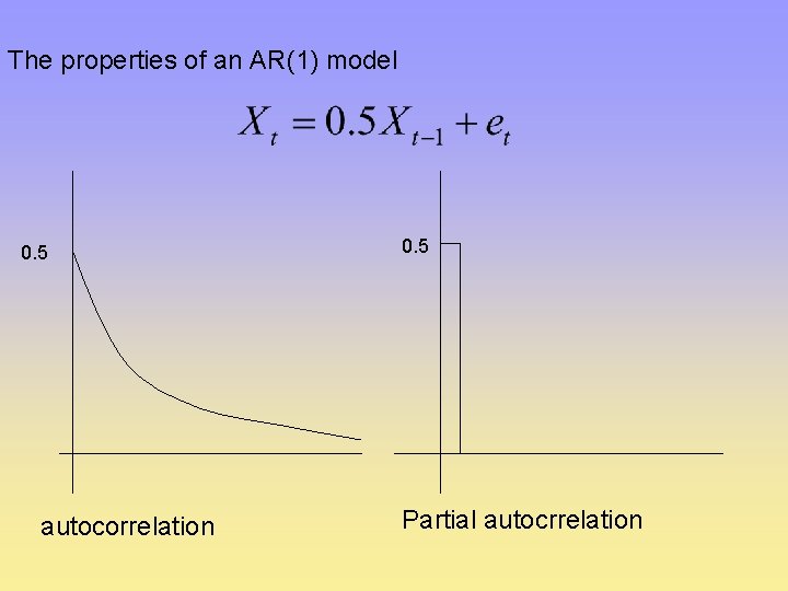
The properties of an AR(1) model 0. 5 autocorrelation 0. 5 Partial autocrrelation

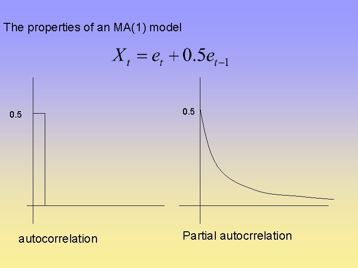
The properties of an MA(1) model 0. 5 autocorrelation 0. 5 Partial autocrrelation

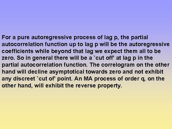
For a pure autoregressive process of lag p, the partial autocorrelation function up to lag p will be the autoregressive coefficients while beyond that lag we expect them all to be zero. So in general there will be a `cut off' at lag p in the partial autocorrelation function. The correlogram on the other hand will decline asymptotical towards zero and not exhibit any discreet `cut of' point. An MA process of order q, on the other hand, will exhibit the reverse property.

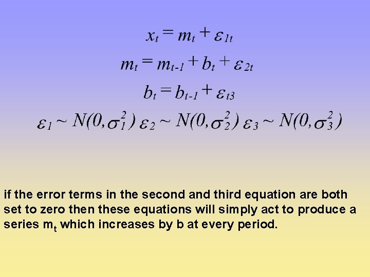
The `Structural Time Series' forecasting model This goes back to the early work of Harrison and Stephens (1971, 1976), but the main proponent of its use in economics and econometrics is Harvey (see among many other references, 1981, 1989). This model may be thought of as a generalisation of the local trend models of Holt, Winter and Brown discussed above. It has a more clearly articulated statistical framework than the earlier models and the notion of an underlying trend can be more easily made precise within this framework.

if the error terms in the second and third equation are both set to zero then these equations will simply act to produce a series mt which increases by b at every period.

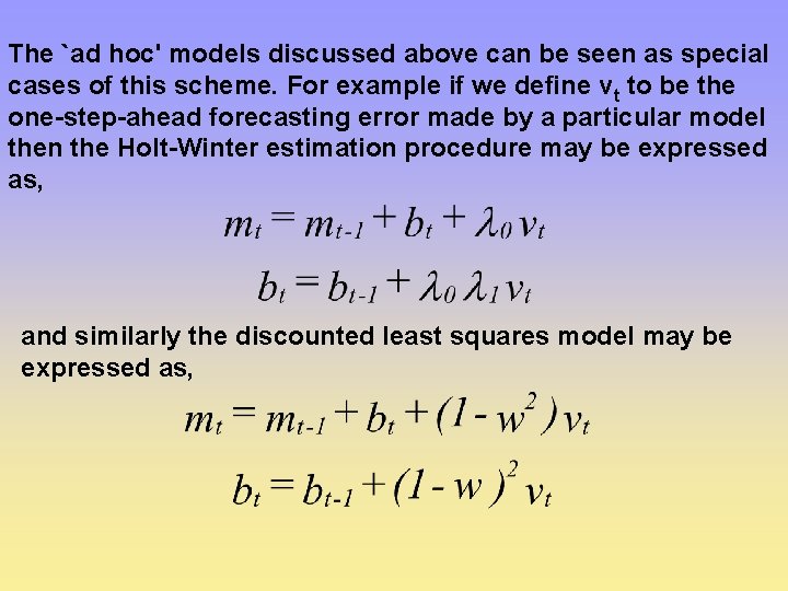
The `ad hoc' models discussed above can be seen as special cases of this scheme. For example if we define vt to be the one-step-ahead forecasting error made by a particular model then the Holt-Winter estimation procedure may be expressed as, and similarly the discounted least squares model may be expressed as,

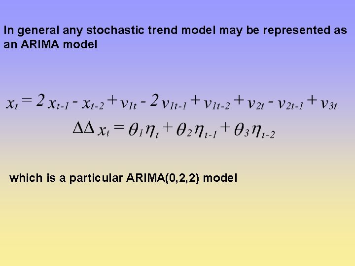
In general any stochastic trend model may be represented as an ARIMA model which is a particular ARIMA(0, 2, 2) model

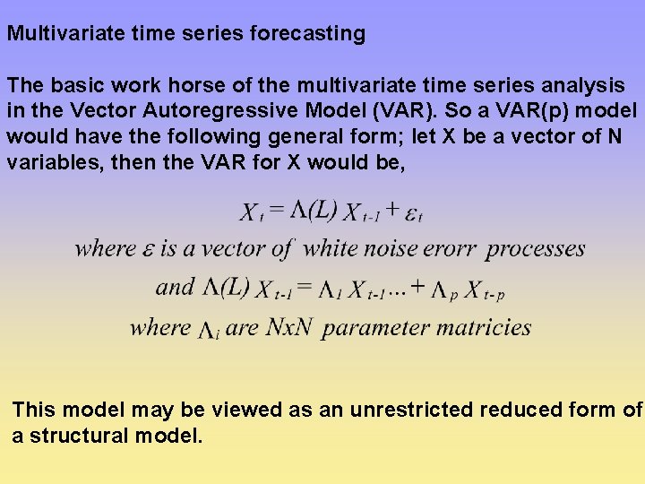
Multivariate time series forecasting The basic work horse of the multivariate time series analysis in the Vector Autoregressive Model (VAR). So a VAR(p) model would have the following general form; let X be a vector of N variables, then the VAR for X would be, This model may be viewed as an unrestricted reduced form of a structural model.

Non-linearities and forecasting • Most of the discussion has been predicated on the assumption of linearity. When this assumption is false many of the basic results still hold. • The Wold representation theorem, for example, still holds. • We can also think of the `ad hoc' local trend models as being local approximations to the true process. • So the preceding analysis is not without value even in the general non-linear case.

But If the true data generating process is non-linear then, in general, any linear forecasting technique will be dominated by the appropriate non-linear model. Chaos A chaotic system is simply a non-linear dynamic system, where, either for all parameter values or for a range of parameter values, the dynamic behaviour of the system is qualitatively different from a linear system. A property of such systems is that even if the true chaotic system is completely deterministic with no measurement error, if we try to model it with standard linear techniques then we will appear to find a linear but stochastic process.

This has raised the fundamental question of whether we are really dealing with a non-linear but deterministic world, rather than the traditional assumption of a linear stochastic one.

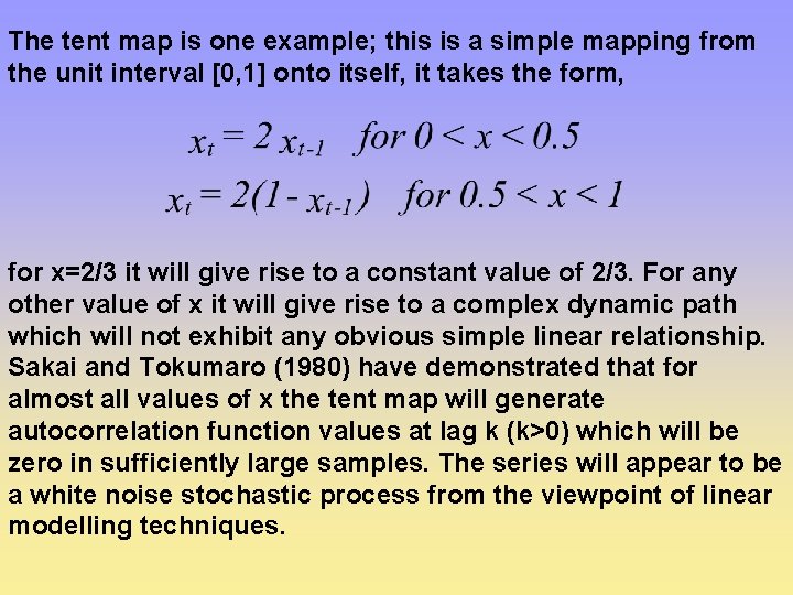
The tent map is one example; this is a simple mapping from the unit interval [0, 1] onto itself, it takes the form, for x=2/3 it will give rise to a constant value of 2/3. For any other value of x it will give rise to a complex dynamic path which will not exhibit any obvious simple linear relationship. Sakai and Tokumaro (1980) have demonstrated that for almost all values of x the tent map will generate autocorrelation function values at lag k (k>0) which will be zero in sufficiently large samples. The series will appear to be a white noise stochastic process from the viewpoint of linear modelling techniques.

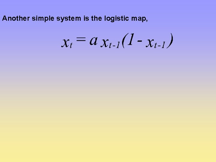
Another simple system is the logistic map,

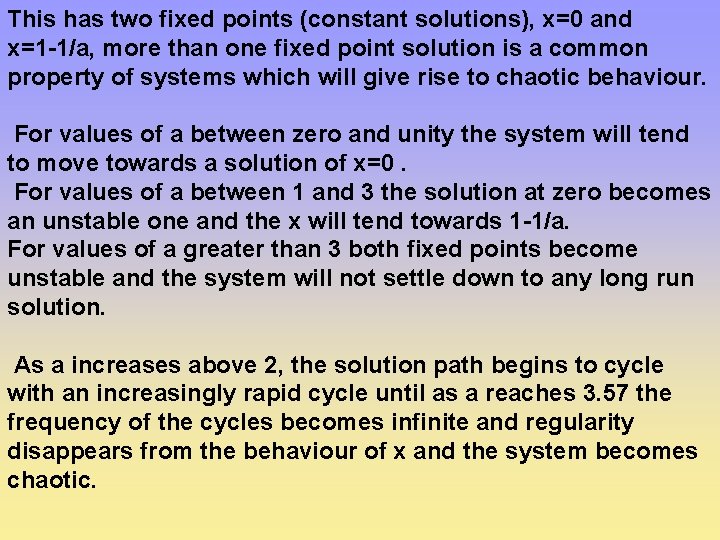
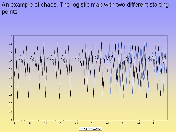
This has two fixed points (constant solutions), x=0 and x=1 -1/a, more than one fixed point solution is a common property of systems which will give rise to chaotic behaviour. For values of a between zero and unity the system will tend to move towards a solution of x=0. For values of a between 1 and 3 the solution at zero becomes an unstable one and the x will tend towards 1 -1/a. For values of a greater than 3 both fixed points become unstable and the system will not settle down to any long run solution. As a increases above 2, the solution path begins to cycle with an increasingly rapid cycle until as a reaches 3. 57 the frequency of the cycles becomes infinite and regularity disappears from the behaviour of x and the system becomes chaotic.

An example of chaos, The logistic map with two different starting points.

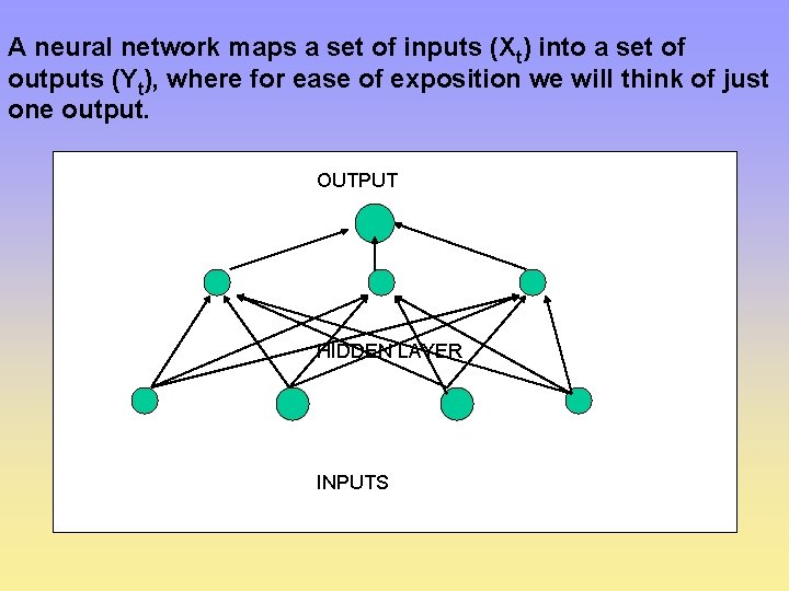
Neural networks Over the last decade a number of techniques have been developed which allow the estimation of general non-linear models without specifying an exact functional form. One of the most popular of these is neural networks. White (1989) has done considerable work recently emphasising the relationship between traditional classical statistics and neural network theory.

A neural network maps a set of inputs (Xt) into a set of outputs (Yt), where for ease of exposition we will think of just one output. OUTPUT HIDDEN LAYER INPUTS

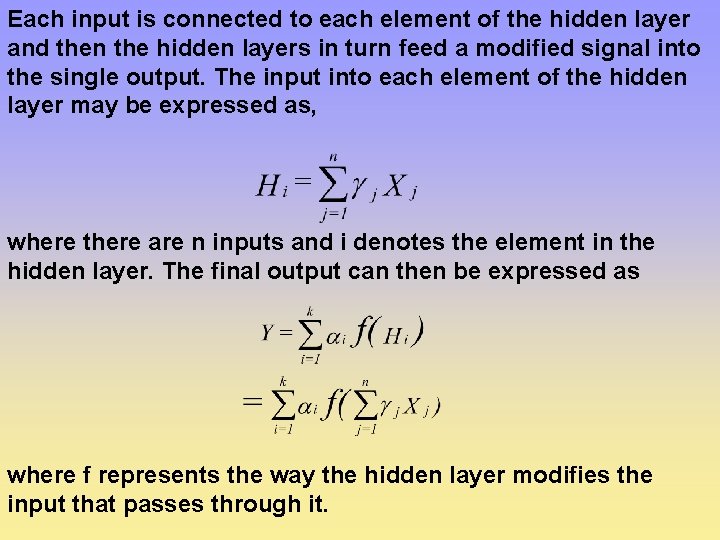
Each input is connected to each element of the hidden layer and then the hidden layers in turn feed a modified signal into the single output. The input into each element of the hidden layer may be expressed as, where there are n inputs and i denotes the element in the hidden layer. The final output can then be expressed as where f represents the way the hidden layer modifies the input that passes through it.

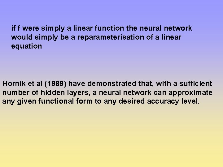
if f were simply a linear function the neural network would simply be a reparameterisation of a linear equation Hornik et al (1989) have demonstrated that, with a sufficient number of hidden layers, a neural network can approximate any given functional form to any desired accuracy level.

selecting the parameters is termed `learning'. It is usually done using a variant on a technique known as `back propagation'. This is related to standard least squares estimation and White(1989) has shown that the two are closely related, although back propagation does not make efficient use of the data.

problems If the data really does have a stochastic element this will mean that the network can achieve a spuriously good fit Given the extreme generality of the functional form large data sets are required for the estimation exercise. Work by White (1989) has emphasised that traditional statistical tools can be brought to bear.