Lecture 2 Probability and Measurement Error Part 1

Lecture 2 Probability and Measurement Error, Part 1

Syllabus Lecture 01 Lecture 02 Lecture 03 Lecture 04 Lecture 05 Lecture 06 Lecture 07 Lecture 08 Lecture 09 Lecture 10 Lecture 11 Lecture 12 Lecture 13 Lecture 14 Lecture 15 Lecture 16 Lecture 17 Lecture 18 Lecture 19 Lecture 20 Lecture 21 Lecture 22 Lecture 23 Lecture 24 Describing Inverse Problems Probability and Measurement Error, Part 1 Probability and Measurement Error, Part 2 The L 2 Norm and Simple Least Squares A Priori Information and Weighted Least Squared Resolution and Generalized Inverses Backus-Gilbert Inverse and the Trade Off of Resolution and Variance The Principle of Maximum Likelihood Inexact Theories Nonuniqueness and Localized Averages Vector Spaces and Singular Value Decomposition Equality and Inequality Constraints L 1 , L∞ Norm Problems and Linear Programming Nonlinear Problems: Grid and Monte Carlo Searches Nonlinear Problems: Newton’s Method Nonlinear Problems: Simulated Annealing and Bootstrap Confidence Intervals Factor Analysis Varimax Factors, Empircal Orthogonal Functions Backus-Gilbert Theory for Continuous Problems; Radon’s Problem Linear Operators and Their Adjoints Fréchet Derivatives Exemplary Inverse Problems, incl. Filter Design Exemplary Inverse Problems, incl. Earthquake Location Exemplary Inverse Problems, incl. Vibrational Problems

Purpose of the Lecture review random variables and their probability density functions introduce correlation and the multivariate Gaussian distribution relate error propagation to functions of random variables

Part 1 random variables and their probability density functions

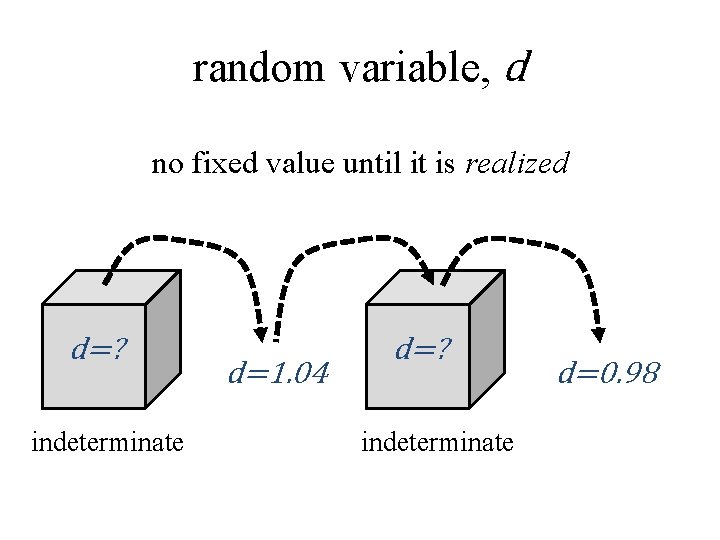
random variable, d no fixed value until it is realized d=? indeterminate d=1. 04 d=? indeterminate d=0. 98

random variables have systematics tendency to takes on some values more often than others

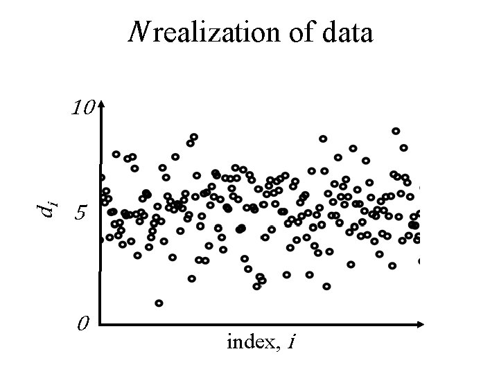
N realization of data di 10 5 0 index, i

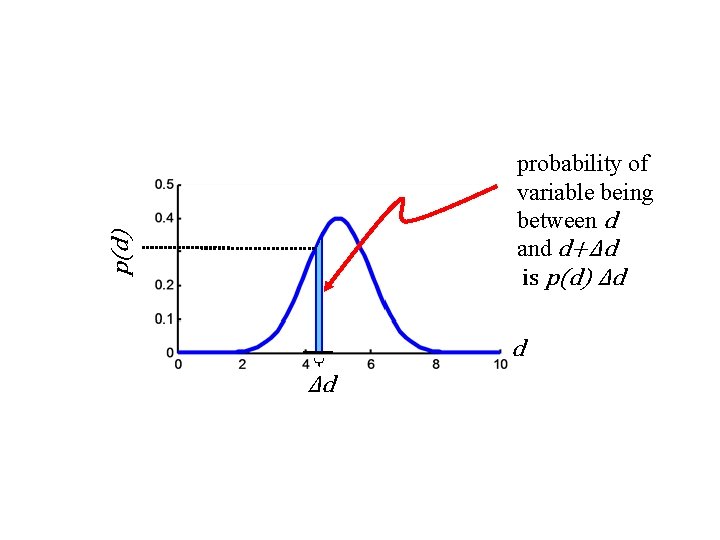
p(d) probability of variable being between d and d+Δd is p(d) Δd d Δd

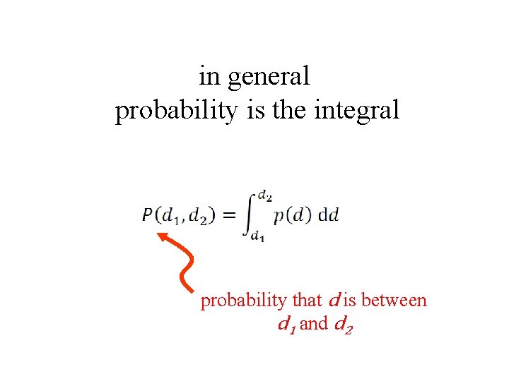
in general probability is the integral probability that d is between d 1 and d 2

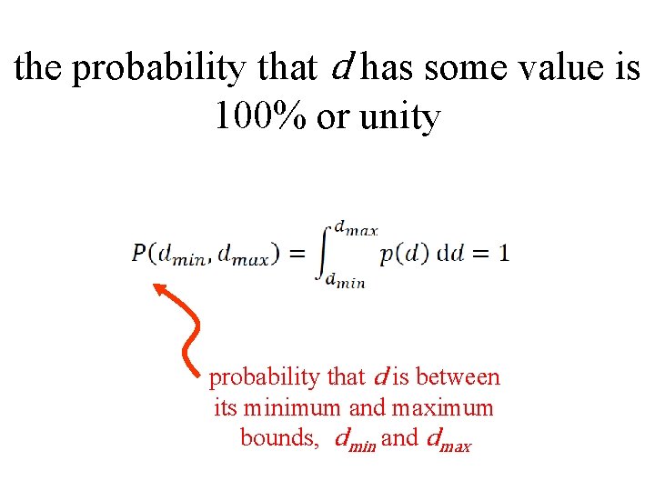
the probability that d has some value is 100% or unity probability that d is between its minimum and maximum bounds, dmin and dmax

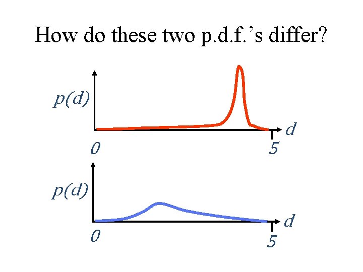
How do these two p. d. f. ’s differ? p(d) d 0 5 p(d) 0 d 5

Summarizing a probability density function typical value “center of the p. d. f. ” amount of scatter around the typical value “width of the p. d. f. ”

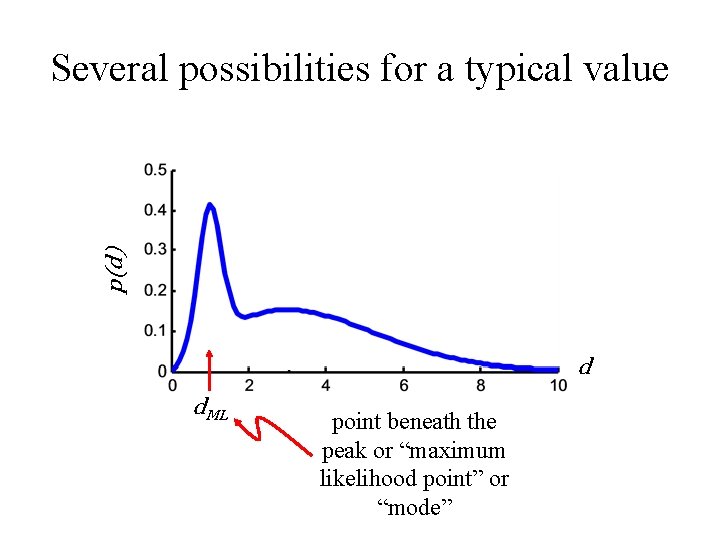
p(d) Several possibilities for a typical value d d. ML point beneath the peak or “maximum likelihood point” or “mode”

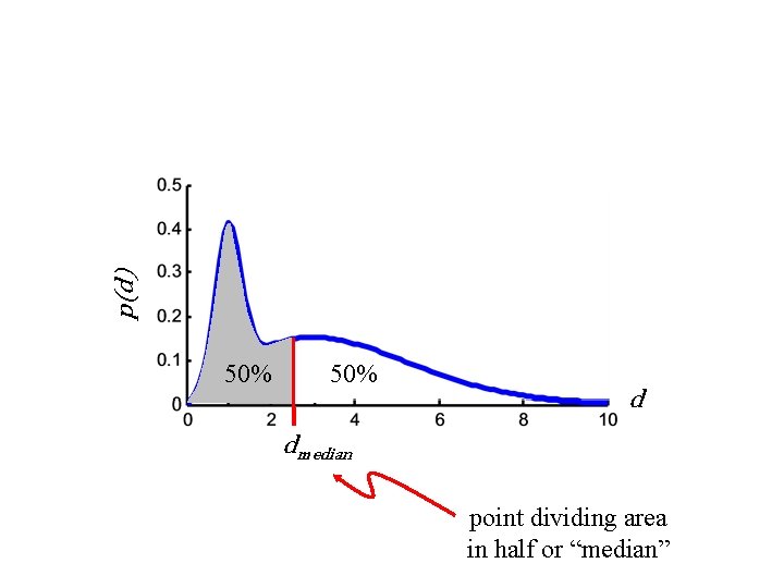
p(d) 50% d dmedian point dividing area in half or “median”

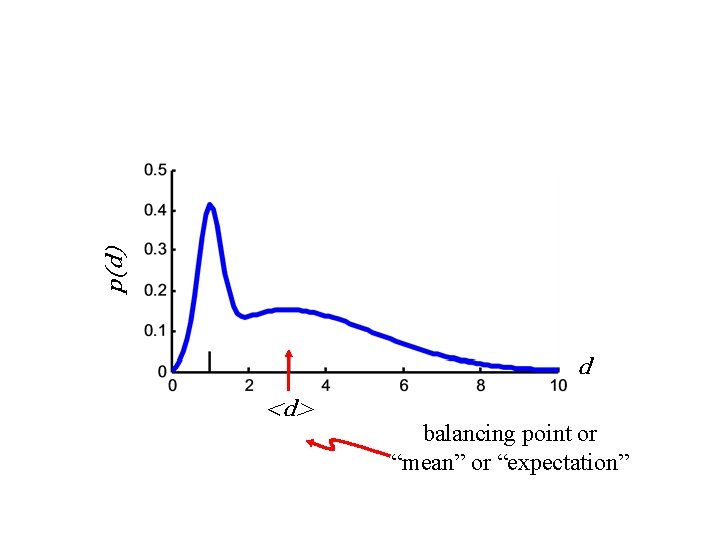
p(d) d <d> balancing point or “mean” or “expectation”

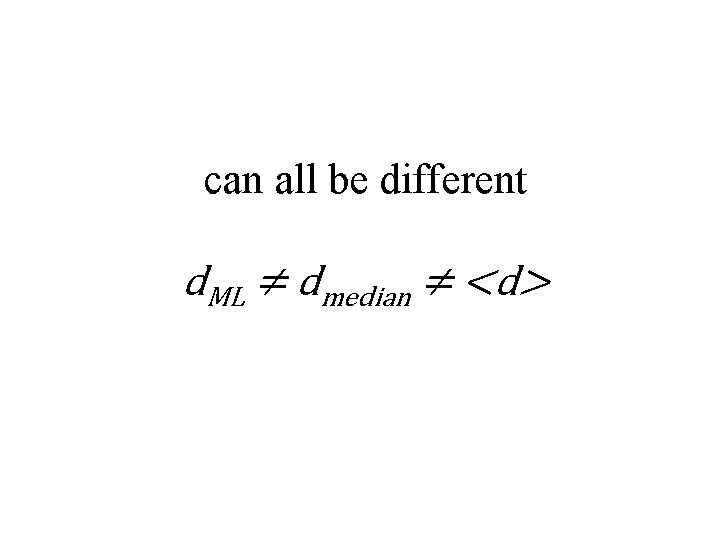
can all be different d. ML ≠ dmedian ≠ <d>

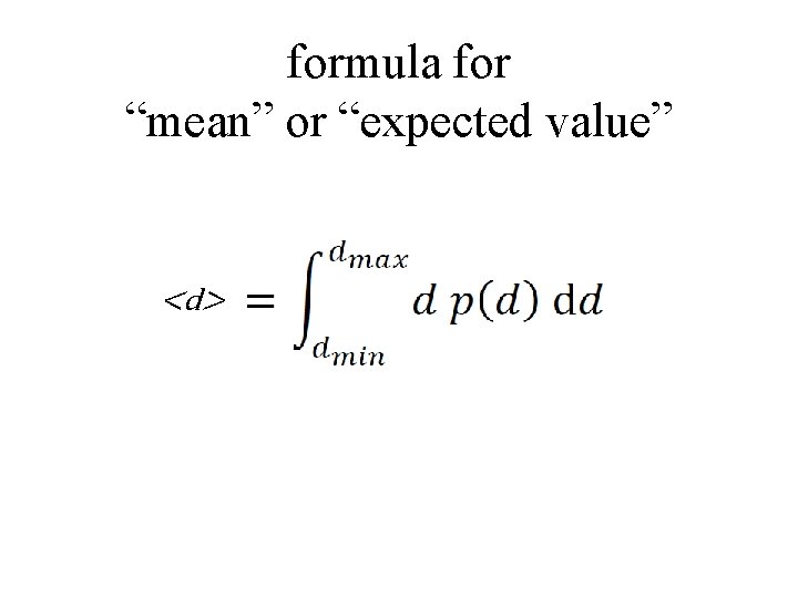
formula for “mean” or “expected value” <d>

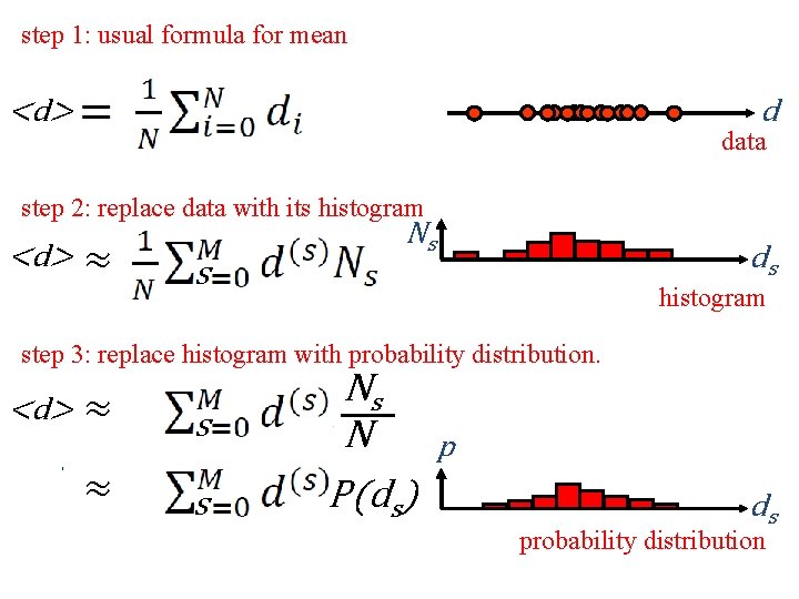
step 1: usual formula for mean d <d> data step 2: replace data with its histogram <d> ≈ s Ns ds histogram step 3: replace histogram with probability distribution. <d> ≈ ≈ s s Ns N P(ds) p ds probability distribution

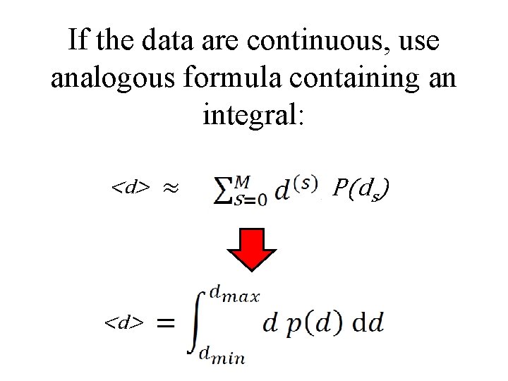
If the data are continuous, use analogous formula containing an integral: <d> ≈ s P(ds)

quantifying width

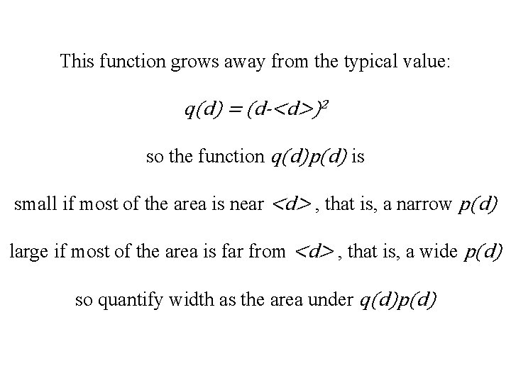
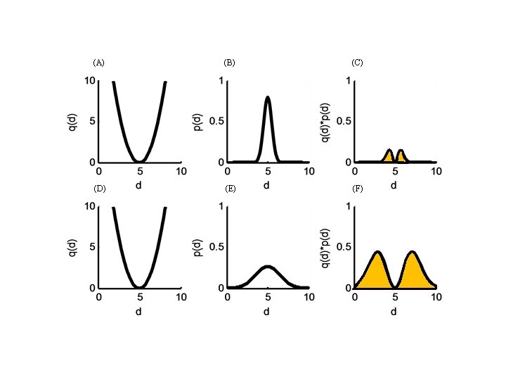
This function grows away from the typical value: q(d) = (d-<d>)2 so the function q(d)p(d) is small if most of the area is near <d> , that is, a narrow p(d) large if most of the area is far from <d> , that is, a wide p(d) so quantify width as the area under q(d)p(d)

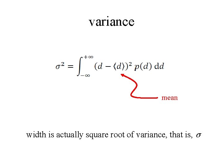
variance mean width is actually square root of variance, that is, σ

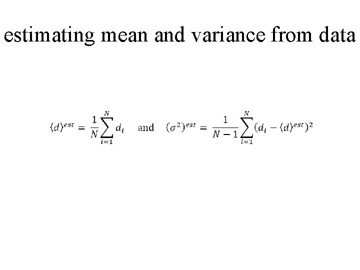
estimating mean and variance from data

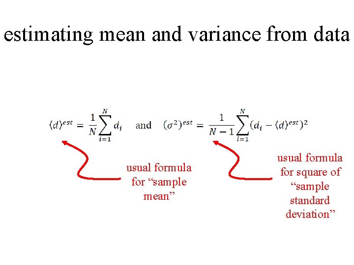
estimating mean and variance from data usual formula for “sample mean” usual formula for square of “sample standard deviation”

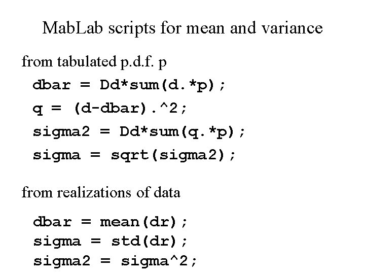
Mab. Lab scripts for mean and variance from tabulated p. d. f. p dbar = Dd*sum(d. *p); q = (d-dbar). ^2; sigma 2 = Dd*sum(q. *p); sigma = sqrt(sigma 2); from realizations of data dbar = mean(dr); sigma = std(dr); sigma 2 = sigma^2;

two important probability density functions: uniform Gaussian (or Normal)

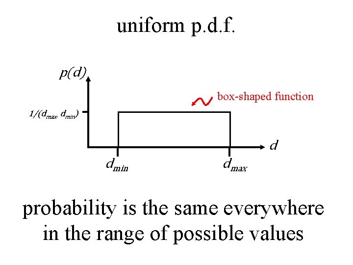
uniform p. d. f. p(d) box-shaped function 1/(dmax- dmin) d dmin dmax probability is the same everywhere in the range of possible values

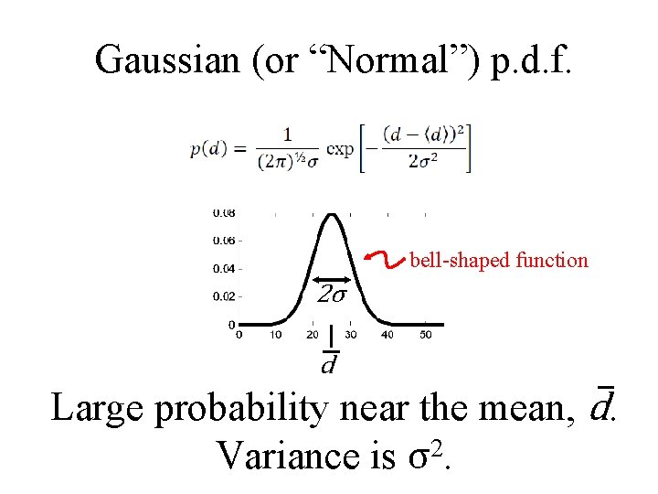
Gaussian (or “Normal”) p. d. f. bell-shaped function 2σ d Large probability near the mean, d. 2 Variance is σ.

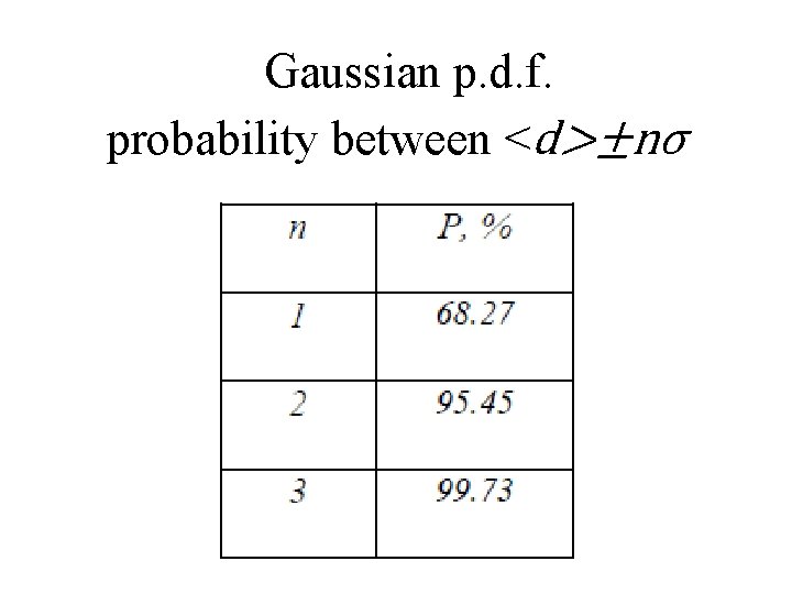
Gaussian p. d. f. probability between <d>±nσ

Part 2 correlated errors

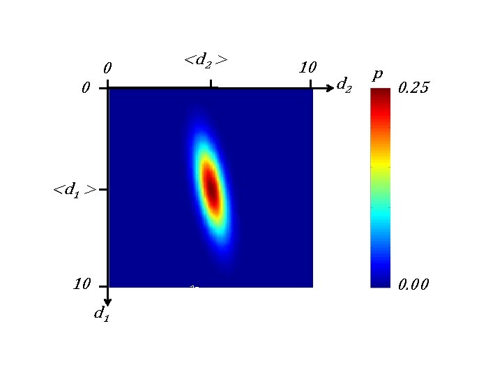
uncorrelated random variables no pattern of between values of one variable and values of another when d 1 is higher than its mean d 2 is higher or lower than its mean with equal probability

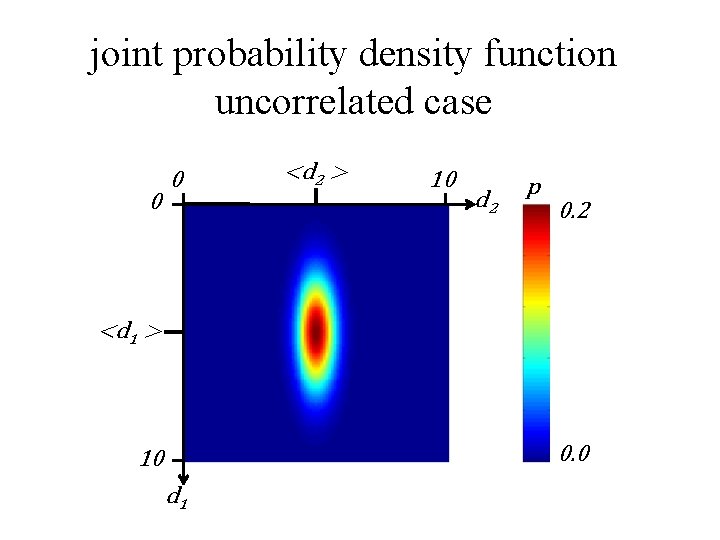
joint probability density function uncorrelated case 0 0 <d 2 > 10 d 2 p 0. 2 <d 1 > 0. 0 10 d 1

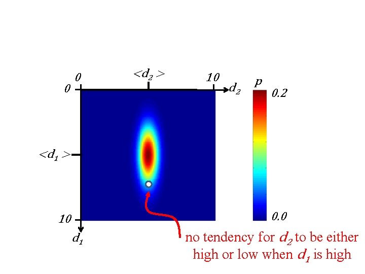
0 0 <d 2 > 10 d 2 p 0. 2 <d 1 > 0. 0 10 d 1 no tendency for d 2 to be either high or low when d 1 is high

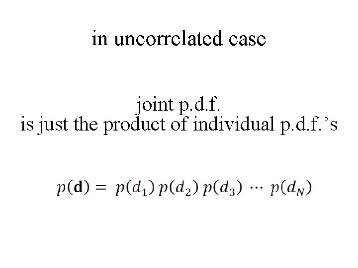
in uncorrelated case joint p. d. f. is just the product of individual p. d. f. ’s

0 <d 2 > 0 10 d 2 p 0. 25 <d 1 > 10 2σ1 d 1 0. 00

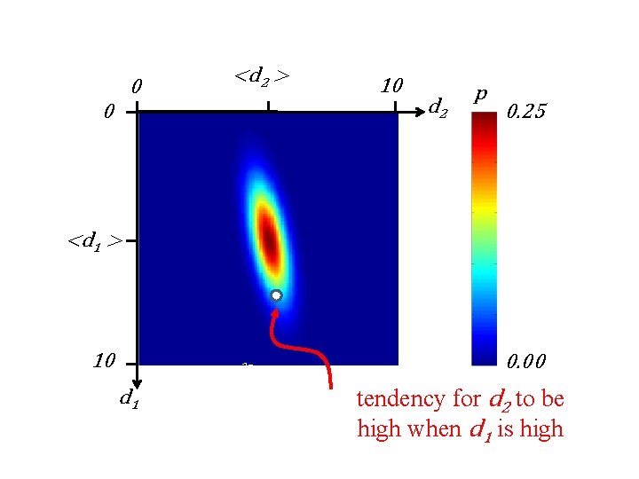
0 <d 2 > 0 10 d 2 p 0. 25 <d 1 > 10 2σ1 d 1 0. 00 tendency for d 2 to be high when d 1 is high

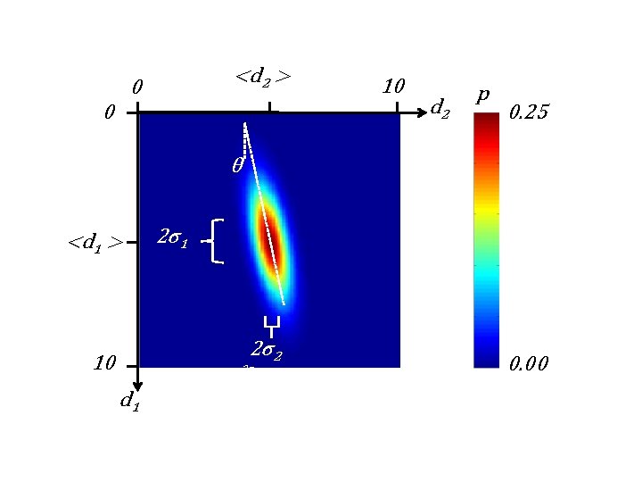
<d 2 > 0 0 10 d 2 p 0. 25 θ <d 1 > 2σ1 2σ2 10 2σ1 d 1 0. 00

<d 2> <d 1> d 2 d 1 2σ1

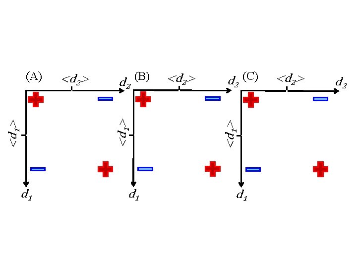
d 1 d 2 (B) d 1 <d 2> d 2 (C) <d 1> <d 2> <d 1> (A) d 1 <d 2> d 2

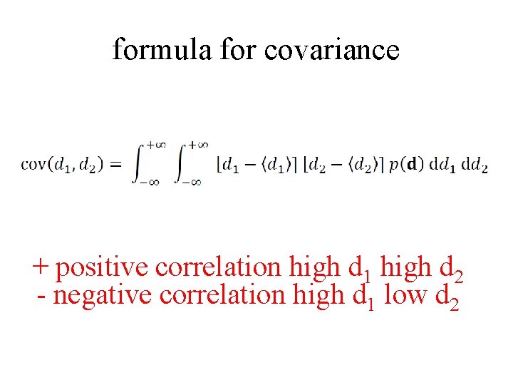
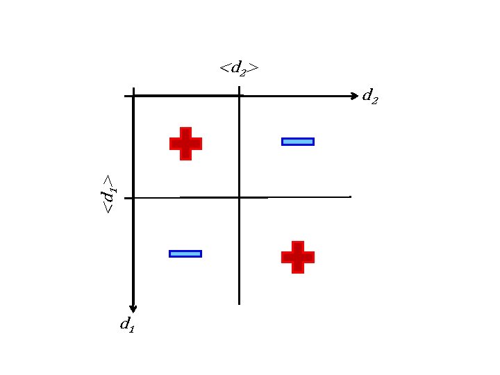
formula for covariance + positive correlation high d 1 high d 2 - negative correlation high d 1 low d 2

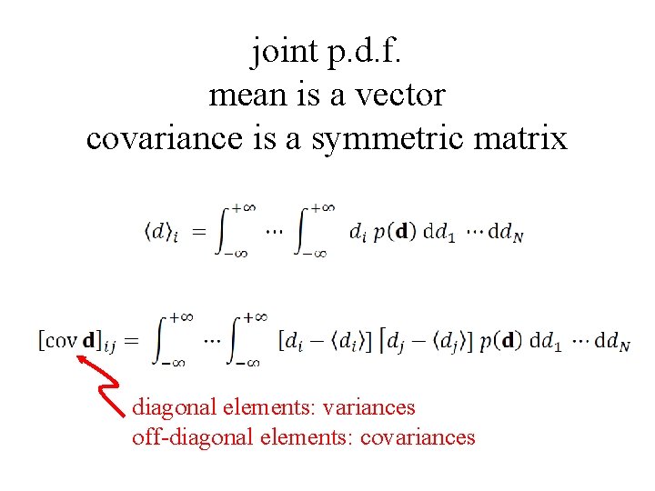
joint p. d. f. mean is a vector covariance is a symmetric matrix diagonal elements: variances off-diagonal elements: covariances

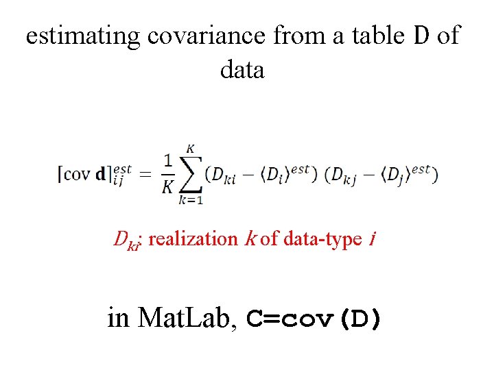
estimating covariance from a table D of data Dki: realization k of data-type i in Mat. Lab, C=cov(D)

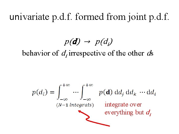
univariate p. d. f. formed from joint p. d. f. p(d) → p(di) behavior of di irrespective of the other ds integrate over everything but di

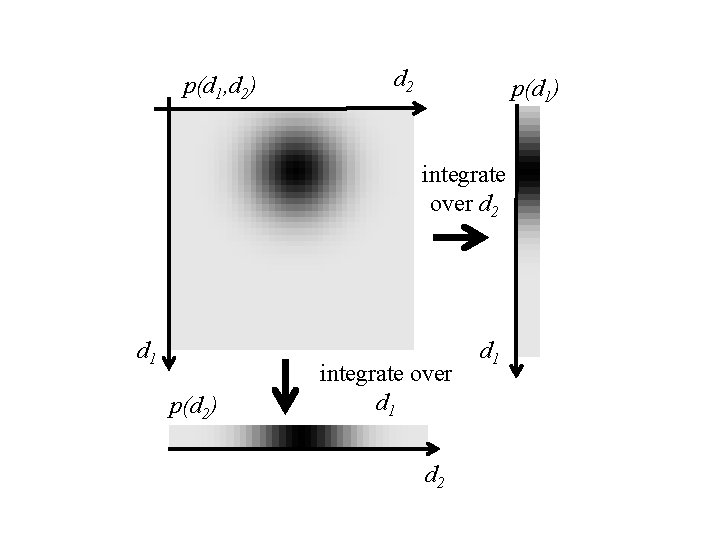
p(d 1, d 2) d 2 p(d 1) integrate over d 2 d 1 p(d 2) integrate over d 1 d 2 d 1

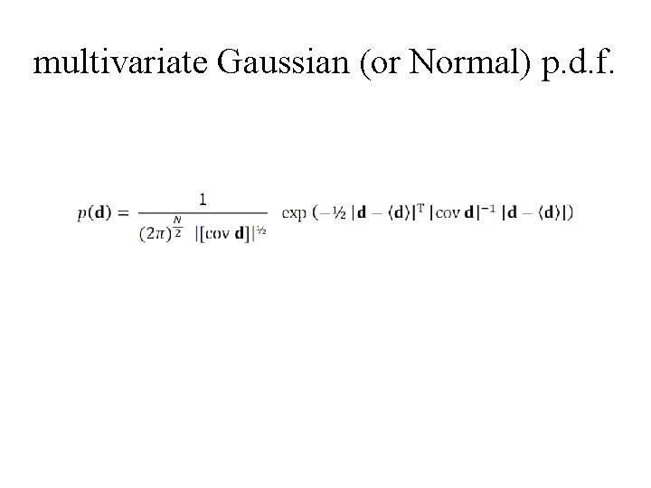
multivariate Gaussian (or Normal) p. d. f.

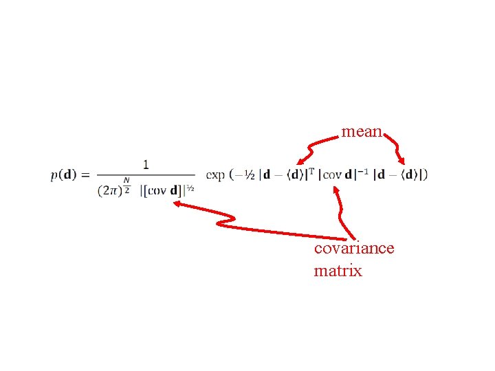
mean covariance matrix

Part 3 functions of random variables

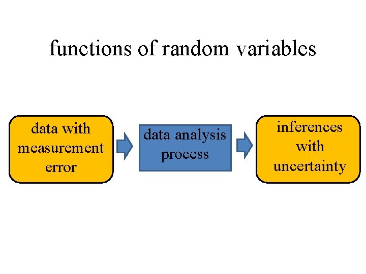
functions of random variables data with measurement error data analysis process inferences with uncertainty

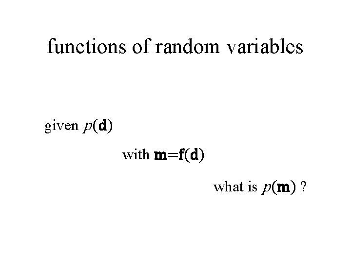
functions of random variables given p(d) with m=f(d) what is p(m) ?

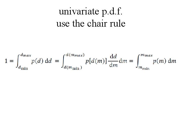
univariate p. d. f. use the chair rule

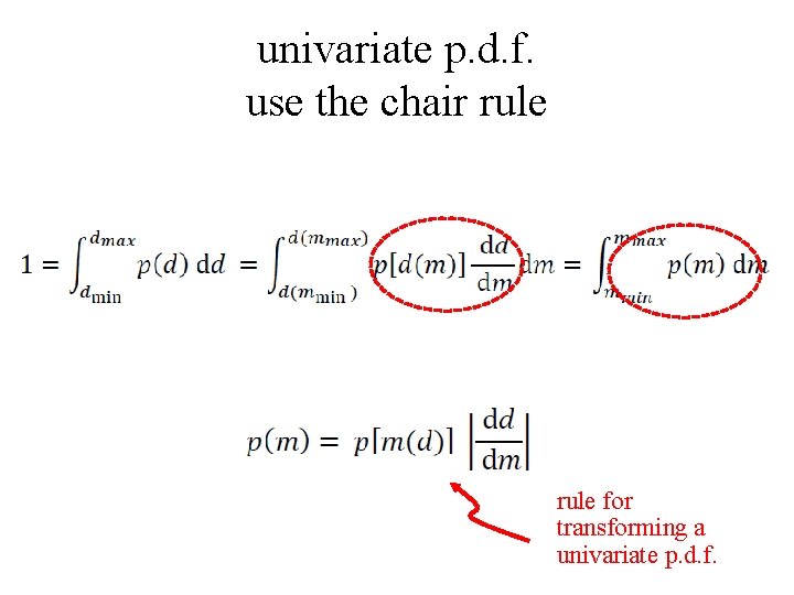
univariate p. d. f. use the chair rule for transforming a univariate p. d. f.

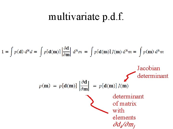
multivariate p. d. f. Jacobian determinant of matrix with elements ∂di/∂mj

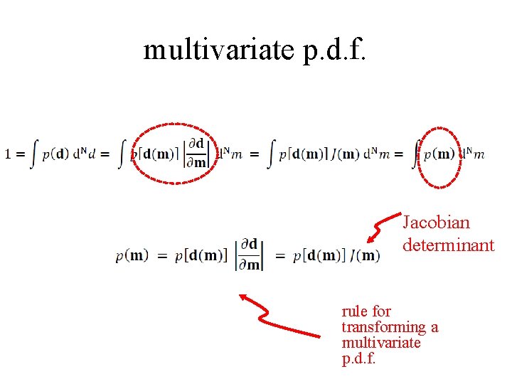
multivariate p. d. f. Jacobian determinant rule for transforming a multivariate p. d. f.

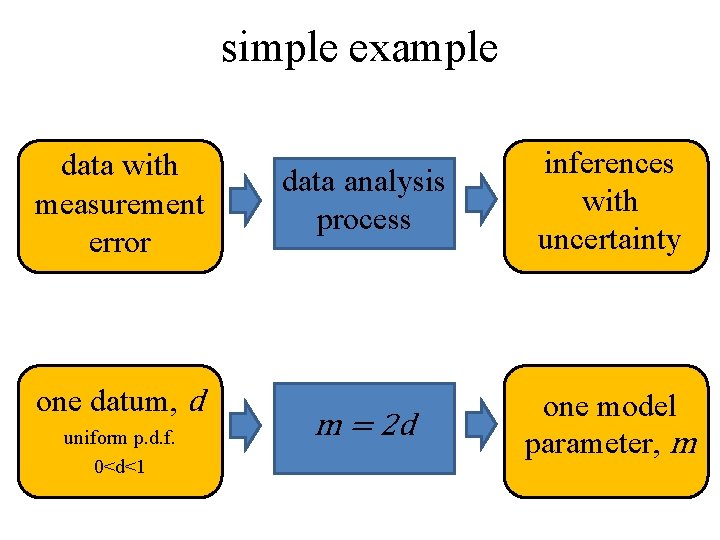
simple example data with measurement error one datum, d uniform p. d. f. 0<d<1 data analysis process inferences with uncertainty m = 2 d one model parameter, m

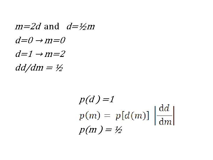
m=2 d and d=½m d=0 → m=0 d=1 → m=2 dd/dm = ½ p(d ) =1 p(m ) = ½

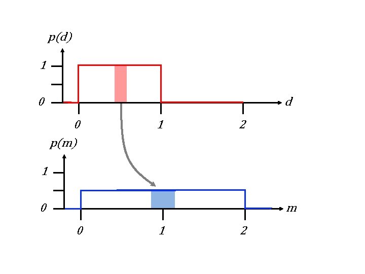
p(d) 1 0 d 0 p(m) 1 2 1 0 m 0 1 2

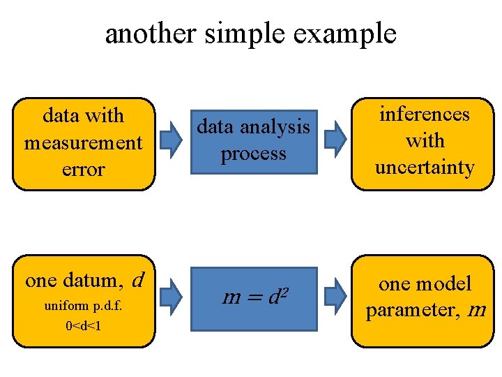
another simple example data with measurement error one datum, d uniform p. d. f. 0<d<1 data analysis process m= d 2 inferences with uncertainty one model parameter, m

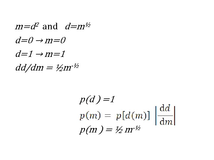
m=d 2 and d=m½ d=0 → m=0 d=1 → m=1 dd/dm = ½m-½ p(d ) =1 p(m ) = ½ m-½

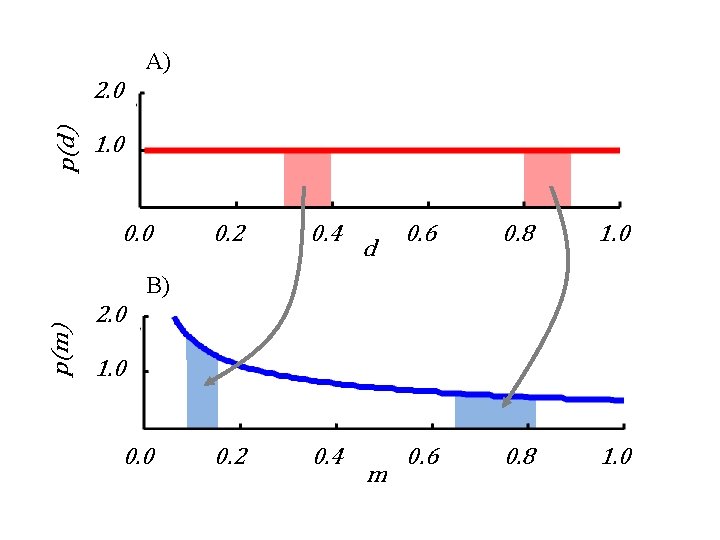
A) p(d) 2. 0 1. 0 0. 2 0. 4 d 0. 6 0. 8 1. 0 p(m) B) 2. 0 1. 0 0. 0 m

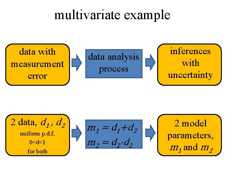
multivariate example data with measurement error 2 data, d 1 , d 2 uniform p. d. f. 0<d<1 for both data analysis process inferences with uncertainty m 1 = d 1+d 2 m 2 = d 2 -d 2 2 model parameters, m 1 and m 2

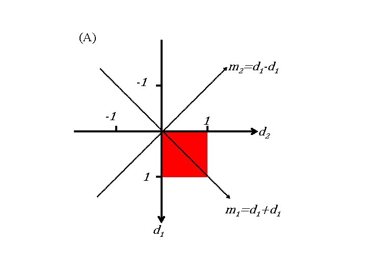
(A) m 2=d 1 -d 1 -1 -1 1 d 2 1 m 1=d 1+d 1

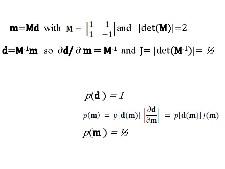
m=Md with and |det(M)|=2 d=M-1 m so ∂d/ ∂ m = M-1 and J= |det(M-1)|= ½ p(d ) = 1 p(m ) = ½

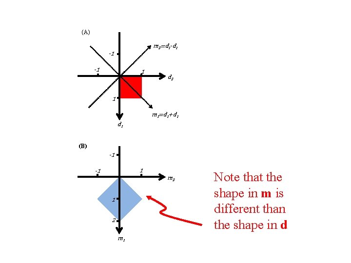
(C) (A) m 2=d 1 -d 1 -1 -1 1 d 2 0 p(d 1) 1 1 m 1=d 1+d 1 d 1 (B) (D) -1 -1 0. 5 m 2 1 1 2 2 m 1 ) Notep(mthat the shape in m is different than the shape in d 0 1 m 1

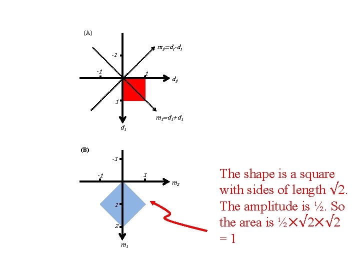
(C) (A) m 2=d 1 -d 1 -1 -1 1 d 2 0 p(d 1) 1 1 m 1=d 1+d 1 d 1 (B) (D) -1 -1 m 2 0 1 1 2 2 m 1 The shape is a square 0. 5 p(m ) with sides of length √ 2. The amplitude is ½. So the area is ½⨉√ 2 =1 1 m 1

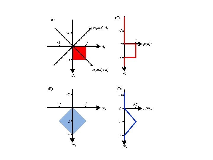
(C) (A) m 2=d 1 -d 1 -1 -1 1 d 2 0 p(d 1) 1 1 m 1=d 1+d 1 d 1 (B) (D) -1 -1 0. 5 m 2 0 1 1 2 2 m 1 p(m 1)

moral p(m) can behavior quite differently from p(d)