Lecture 2 Key Functions and Parametric Distributions Survival
Lecture 2: Key Functions and Parametric Distributions Survival Function Hazard Function Median Survival Common Parametric Distributions
But First • Let’s think a little more about censoring and truncation using an example… • An investigator is interested in determining if treatment with amoxetine leads to recovery of cognitive function in rats with brain lesions that mimic Parkinson’s disease. • The outcome of interest is time to “complete” recovery of cognitive function – i. e. time it takes to return to baseline cognitive function after treatment with amoxetine.
Amoxetine and Cognitive Function • Collect baseline measure of cognitive function – Time to correctly perform water radial arm maze (WRAM) task • Induce cognitive impairment – Treat 4 week old rats with N-(2 -chloroethyl)-N-ethyl-bromobenzylamine (DSP-4) – causes noradrenergic lesions in the locus coeruleus. • Treat lesioned animals with Amoxetine – daily dose for 4 weeks (ages 4 to 8 weeks) – 0, 0. 3, 1. 0, or 3. 0 mg/kg • Measures cognitive performance post treatment – weekly for 16 weeks (ages 8 to 24 weeks) – Endpoint: time it takes reach >75% baseline cognitive function
Describe the type of censoring • Rat survives to 24 weeks of age but never achieves complete cognitive recovery • Rat does not achieve complete cognitive recovery at 12 weeks but does by 13 weeks • Rat that dies at 16 weeks but has not yet achieve complete cognitive recovery
Describe the type of censoring • Rat doesn’t develop brain lesions due to misplaced DSP-4 treatment and shows complete cognitive recovery at 8 weeks • Rat shows complete cognitive recovery 8 at weeks
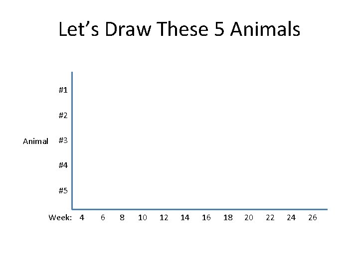
Let’s Draw These 5 Animals #1 #2 Animal #3 #4 #5 Week: 4 6 8 10 12 14 16 18 20 22 24 26
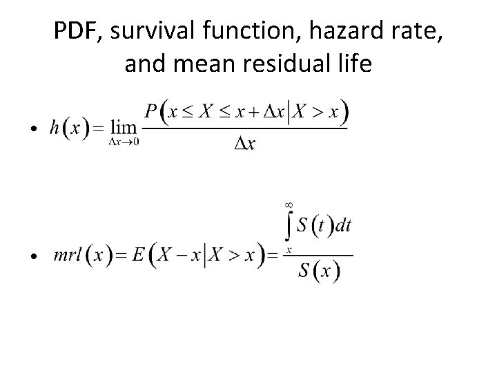
Time to Event Outcomes • Modeled using “survival analysis” • Define X = time to event – X is a random variable – Realizations of X are denoted x – X>0 • Key characterizing functions – – Survival function Hazard rate (or function) Probability density function Mean residual life
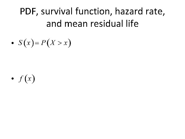
PDF, survival function, hazard rate, and mean residual life • •
PDF, survival function, hazard rate, and mean residual life • •
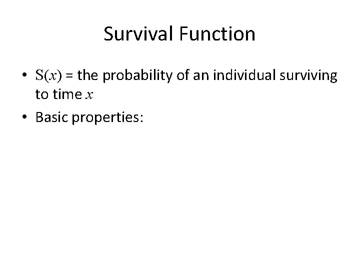
Survival Function • S(x) = the probability of an individual surviving to time x • Basic properties:
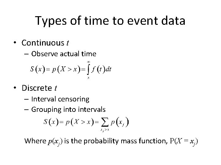
Types of time to event data • Continuous t – Observe actual time • Discrete t – Interval censoring – Grouping into intervals Where p(xj) is the probability mass function, P(X = xj)
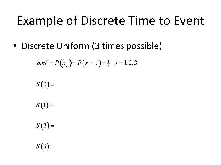
Example of Discrete Time to Event • Discrete Uniform (3 times possible)
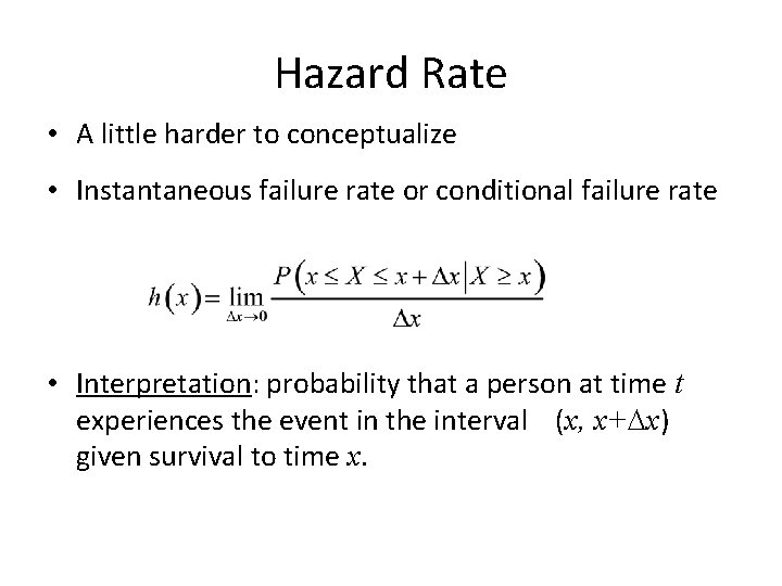
Hazard Rate • A little harder to conceptualize • Instantaneous failure rate or conditional failure rate • Interpretation: probability that a person at time t experiences the event in the interval (x, x+Dx) given survival to time x.
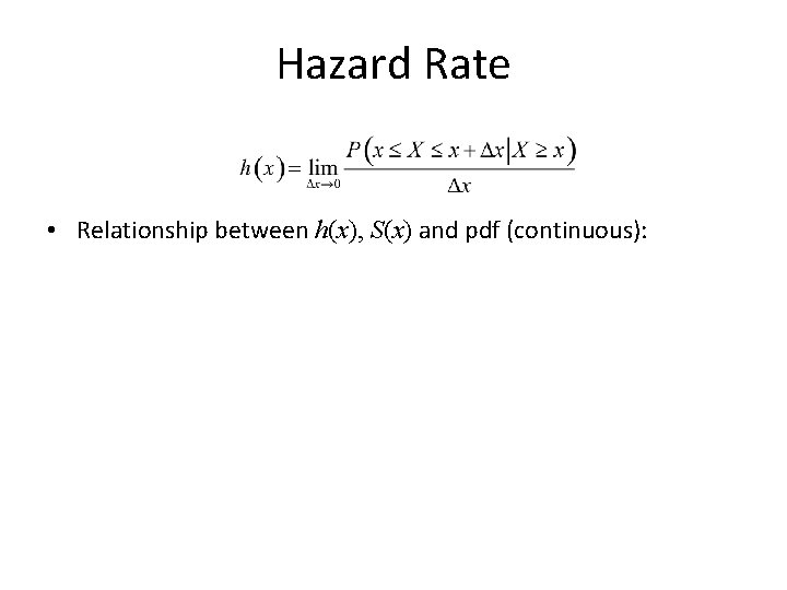
Hazard Rate • Relationship between h(x), S(x) and pdf (continuous):
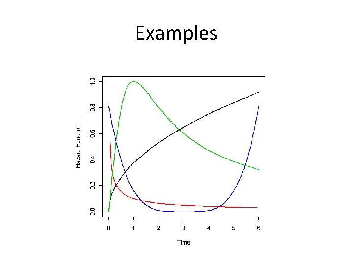
Hazard Function • Useful for conceptualizing how the chance of an event changes over time • i. e. consider hazard ‘relative’ over time • Examples: – Treatment related mortality • Early on, high risk of death • Later on, risk of death decreases – Aging • Early on, low risk of death • Later on, high risk of death
Shapes of Hazard Functions • Increasing – Natural aging and wear • Decreasing – Early failures due to device or transplant failures • Bathtub – Populations followed from birth • Hump Shaped – Initial risk of event, followed by decreasing chance of event
Examples
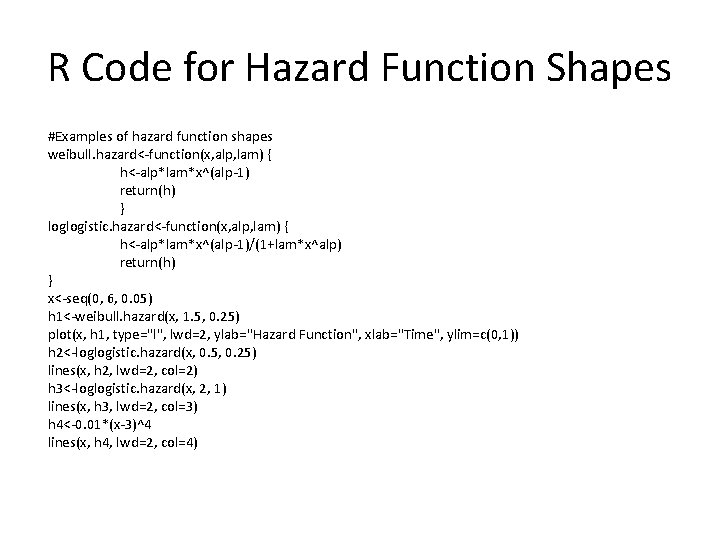
R Code for Hazard Function Shapes #Examples of hazard function shapes weibull. hazard<-function(x, alp, lam) { h<-alp*lam*x^(alp-1) return(h) } loglogistic. hazard<-function(x, alp, lam) { h<-alp*lam*x^(alp-1)/(1+lam*x^alp) return(h) } x<-seq(0, 6, 0. 05) h 1<-weibull. hazard(x, 1. 5, 0. 25) plot(x, h 1, type="l", lwd=2, ylab="Hazard Function", xlab="Time", ylim=c(0, 1)) h 2<-loglogistic. hazard(x, 0. 5, 0. 25) lines(x, h 2, lwd=2, col=2) h 3<-loglogistic. hazard(x, 2, 1) lines(x, h 3, lwd=2, col=3) h 4<-0. 01*(x-3)^4 lines(x, h 4, lwd=2, col=4)
Cumulative Hazard Function • Often used instead of the hazard function – Relationship between H(x) and S(x) • More on this later or model checking…
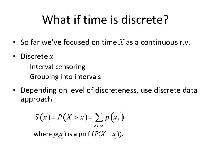
What if time is discrete? • So far we’ve focused on time X as a continuous r. v. • Discrete x – Interval censoring – Grouping into intervals • Depending on level of discreteness, use discrete data approach where p(xj) is a pmf (P(X = xj)).
Complications • How can we use this to define our “discrete” hazard function?
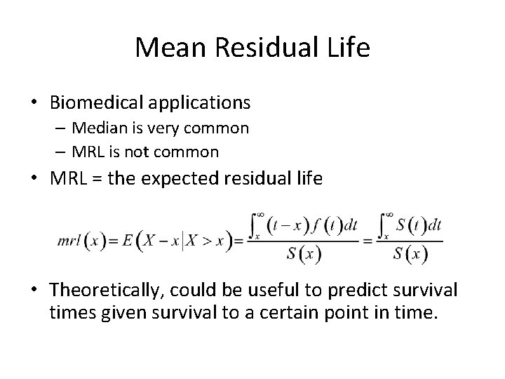
Mean Residual Life • Biomedical applications – Median is very common – MRL is not common • MRL = the expected residual life • Theoretically, could be useful to predict survival times given survival to a certain point in time.
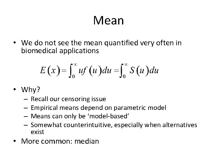
Mean • We do not see the mean quantified very often in biomedical applications • Why? – – Recall our censoring issue Empirical means depend on parametric model Means can only be ‘model-based’ Somewhat counterintuitive, especially when alternatives exist • More common: median
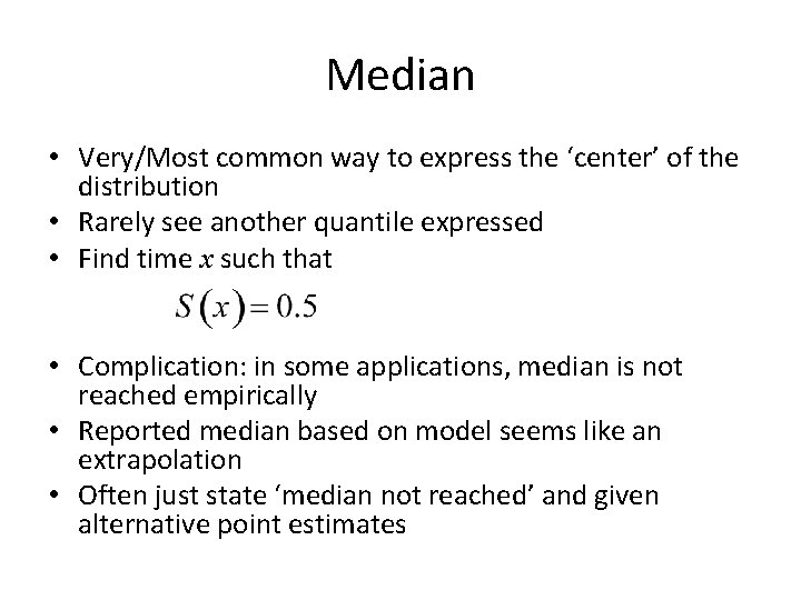
Median • Very/Most common way to express the ‘center’ of the distribution • Rarely see another quantile expressed • Find time x such that • Complication: in some applications, median is not reached empirically • Reported median based on model seems like an extrapolation • Often just state ‘median not reached’ and given alternative point estimates
X-Year Survival Rate • Many applications have ‘landmark’ times that historically used to quantify survival • Examples: – Breast cancer: 5 year relapse-free survival – Pancreatic cancer: 6 month survival – Acute myeloid leukemia (AML): 12 month relapsefree survival • Solve for S(x) given x
Common Parametric Distributions • Course will focus on non-parametric and semiparametric methods • But… some parametrics can be useful • Especially for trial design • Note that power and precision are improved under parametric approaches versus others
Example 1: Exponential • Recall the exponential distribution – f(x) = – F(x) = • What is S(x) based on F(x) and f(x) – S(x) =
Example 1: Exponential • What about H(x) and h(x) – H(x) = – h(x) = • l represents the failure rate per unit of time – Large l, rapid decay – Small l, slow decay

Example 1: Exponential
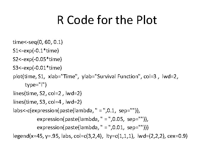
R Code for the Plot time<-seq(0, 60, 0. 1) S 1<-exp(-0. 1*time) S 2<-exp(-0. 05*time) S 3<-exp(-0. 01*time) plot(time, S 1, xlab="Time", ylab="Survival Function", col=3 , lwd=2, type="l") lines(time, S 2, col=2 , lwd=2) lines(time, S 3, col=4 , lwd=2) labs<-c(expression(paste(lambda, " = ", 0. 1, sep="")), expression(paste(lambda, " = ", 0. 05, sep="")), expression(paste(lambda, " = ", 0. 01, sep=""))) legend(x=45, y=. 95, labs, col=c(3, 2, 4), lty=c(1, 1, 1), lwd=(2, 2, 2), cex=0. 9)
Example: Kidney Infection after Catheterization • Kidney infection after catheter insertion in patients using portable dialysis equipment • Time to event = time to catheter removal – BUT the catheter can be removed for reasons other than infection (right censored) • Only 76 observations (!) • Time to infection is outcome of interest • Question: can we describe it using a parametric approach?
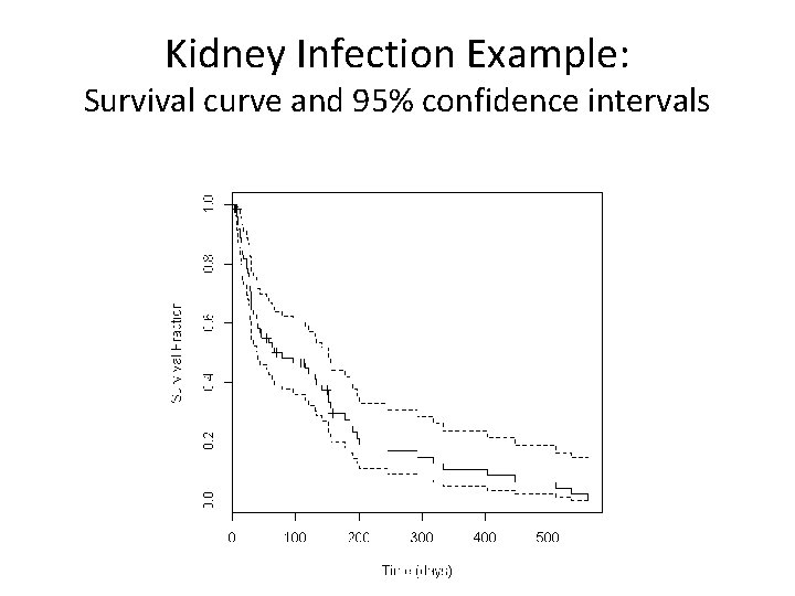
Kidney Infection Example: Survival curve and 95% confidence intervals
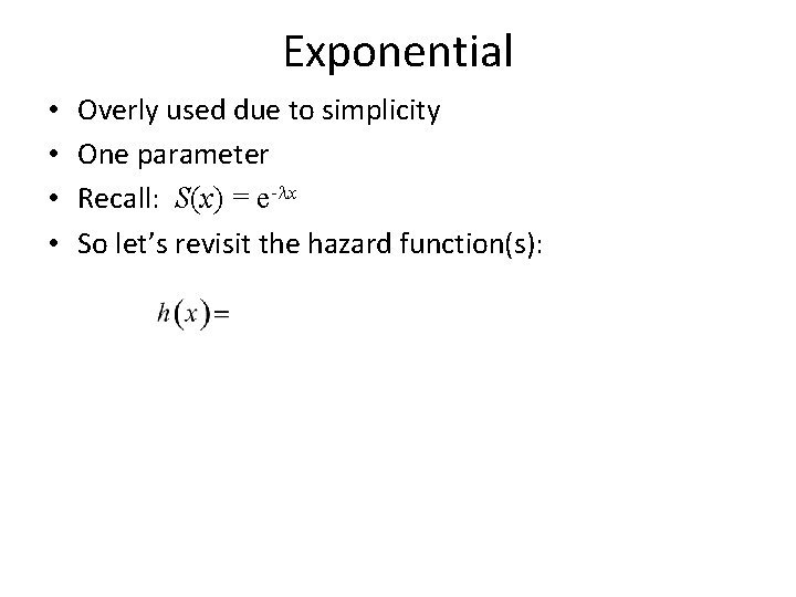
Exponential • • Overly used due to simplicity One parameter Recall: S(x) = e-lx So let’s revisit the hazard function(s):
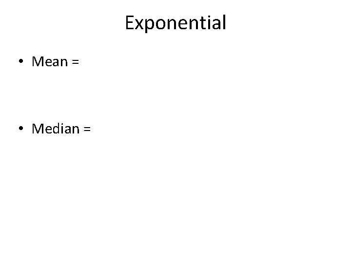
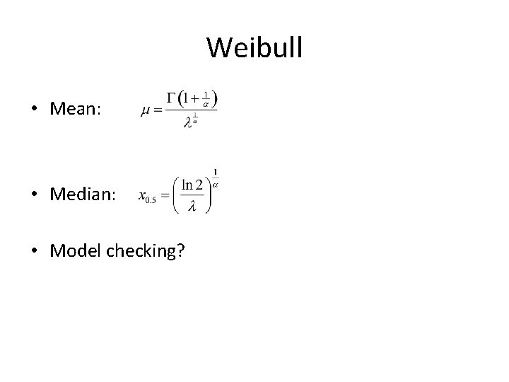
Exponential • Mean = • Median =
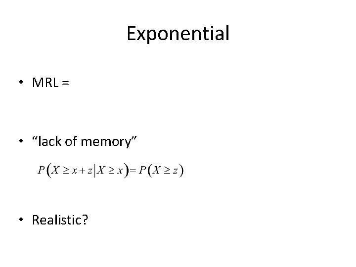
Exponential • MRL = • “lack of memory” • Realistic?
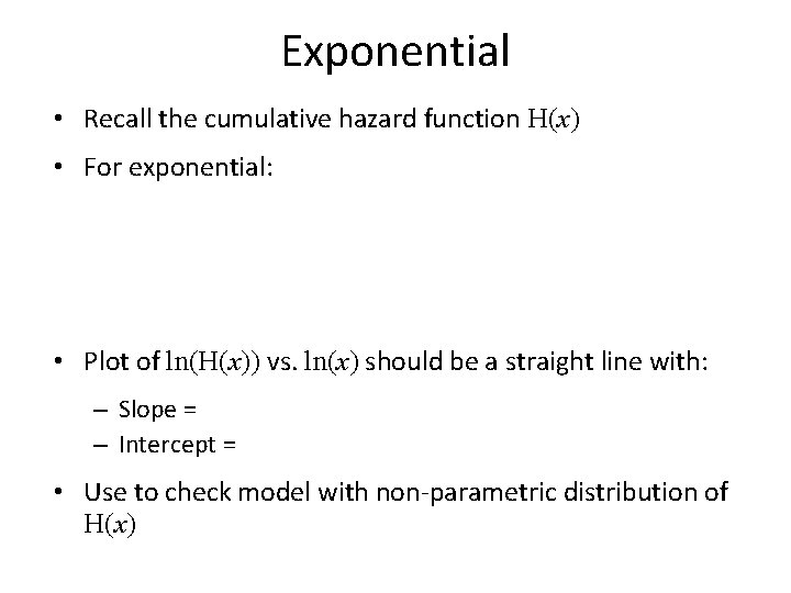
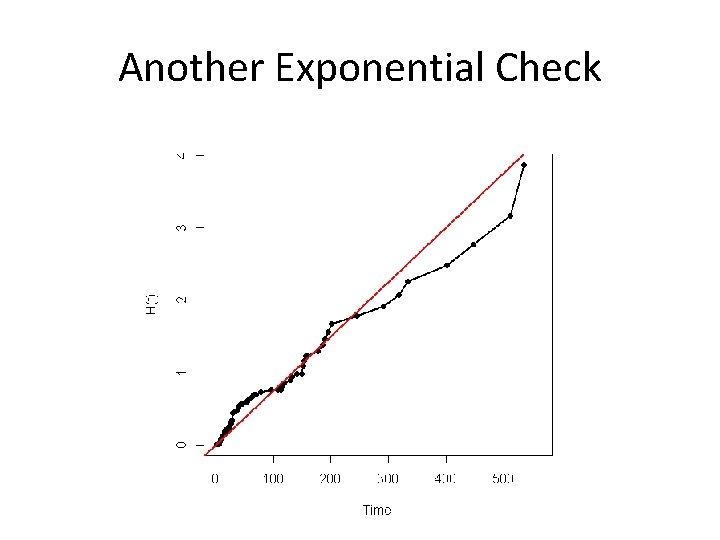
Exponential • Recall the cumulative hazard function H(x) • For exponential: • Plot of ln(H(x)) vs. ln(x) should be a straight line with: – Slope = – Intercept = • Use to check model with non-parametric distribution of H(x)
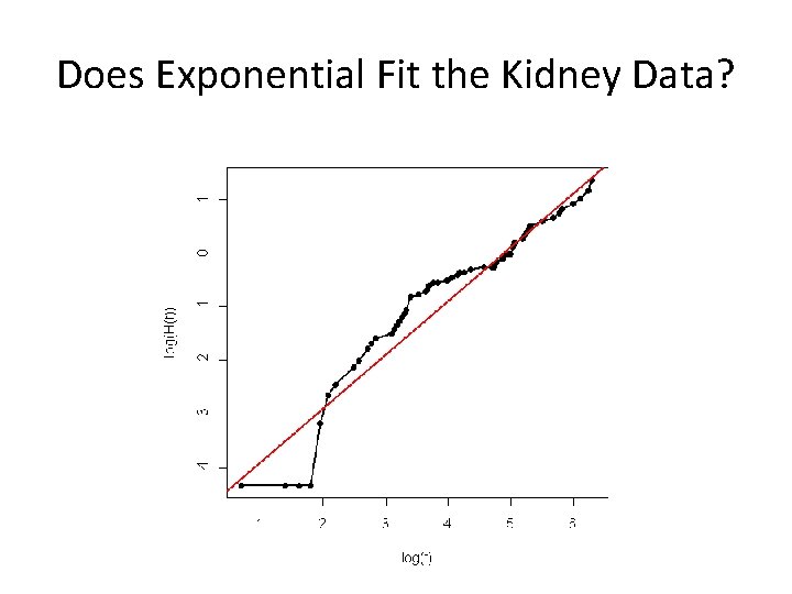
Does Exponential Fit the Kidney Data?
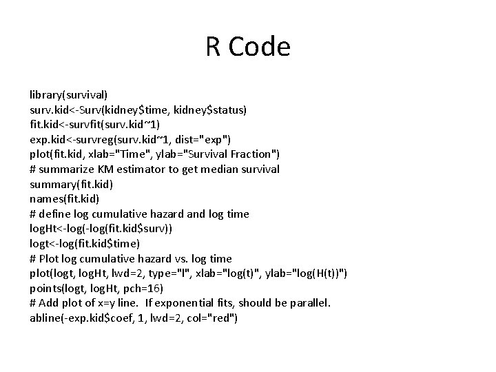
R Code library(survival) surv. kid<-Surv(kidney$time, kidney$status) fit. kid<-survfit(surv. kid~1) exp. kid<-survreg(surv. kid~1, dist="exp") plot(fit. kid, xlab="Time", ylab="Survival Fraction") # summarize KM estimator to get median survival summary(fit. kid) names(fit. kid) # define log cumulative hazard and log time log. Ht<-log(fit. kid$surv)) logt<-log(fit. kid$time) # Plot log cumulative hazard vs. log time plot(logt, log. Ht, lwd=2, type="l", xlab="log(t)", ylab="log(H(t))") points(logt, log. Ht, pch=16) # Add plot of x=y line. If exponential fits, should be parallel. abline(-exp. kid$coef, 1, lwd=2, col="red")
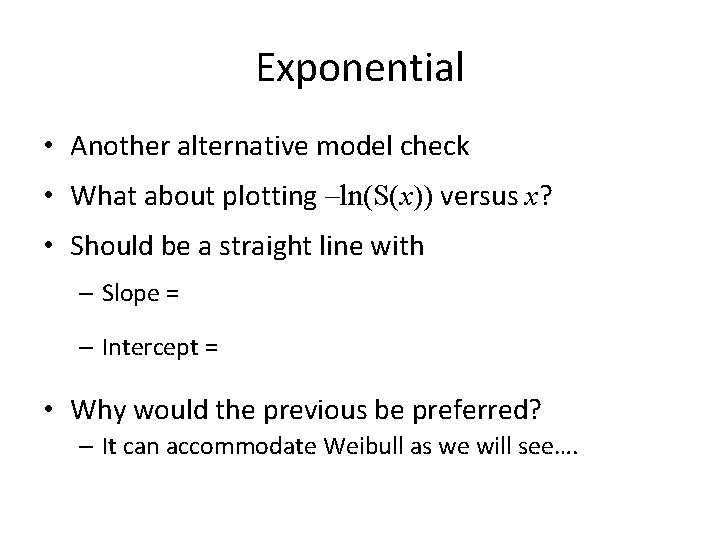
Exponential • Another alternative model check • What about plotting –ln(S(x)) versus x? • Should be a straight line with – Slope = – Intercept = • Why would the previous be preferred? – It can accommodate Weibull as we will see….
Another Exponential Check
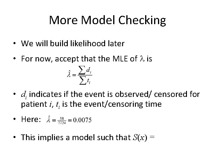
More Model Checking • We will build likelihood later • For now, accept that the MLE of l is • di indicates if the event is observed/ censored for patient i, ti is the event/censoring time • Here: • This implies a model such that S(x) =
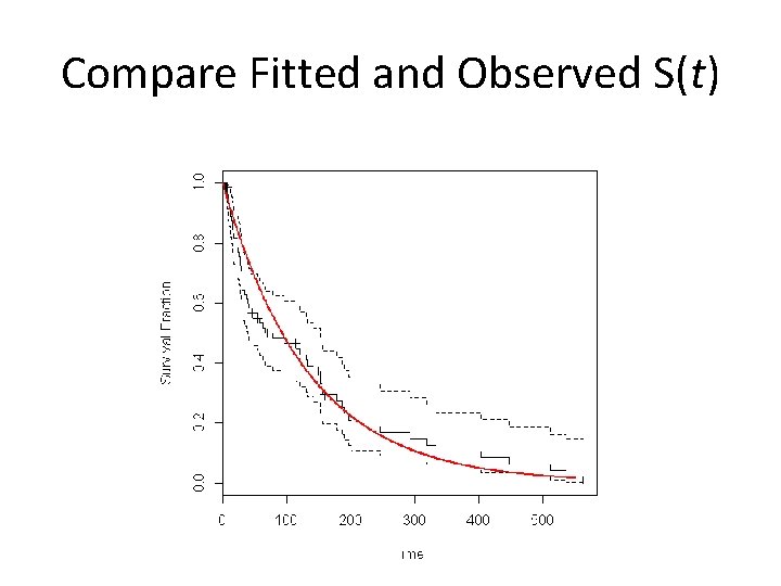
Compare Fitted and Observed S(t)
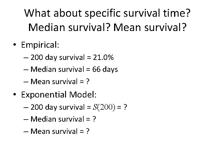
What about specific survival time? Median survival? Mean survival? • Empirical: – 200 day survival = 21. 0% – Median survival = 66 days – Mean survival = ? • Exponential Model: – 200 day survival = S(200) = ? – Median survival = ? – Mean survival = ?
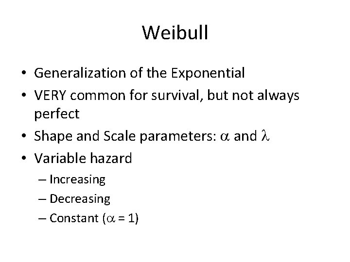
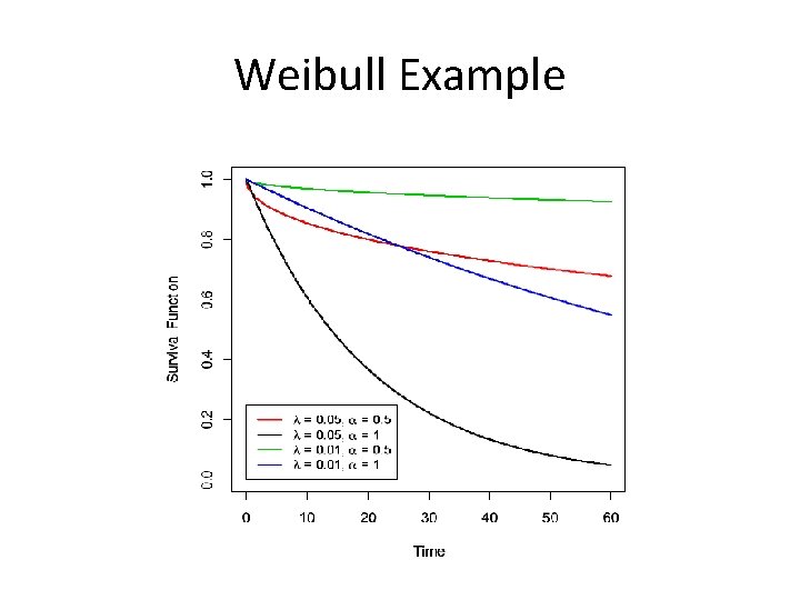
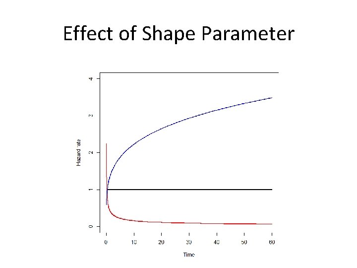
Weibull • Generalization of the Exponential • VERY common for survival, but not always perfect • Shape and Scale parameters: a and l • Variable hazard – Increasing – Decreasing – Constant (a = 1)
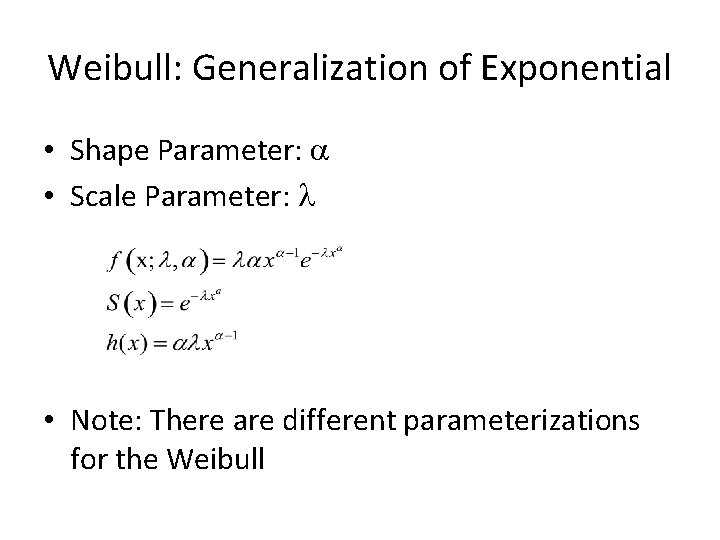
Weibull: Generalization of Exponential • Shape Parameter: a • Scale Parameter: l • Note: There are different parameterizations for the Weibull
Weibull Example
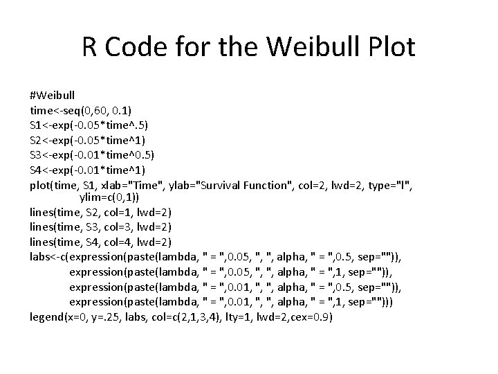
R Code for the Weibull Plot #Weibull time<-seq(0, 60, 0. 1) S 1<-exp(-0. 05*time^. 5) S 2<-exp(-0. 05*time^1) S 3<-exp(-0. 01*time^0. 5) S 4<-exp(-0. 01*time^1) plot(time, S 1, xlab="Time", ylab="Survival Function", col=2, lwd=2, type="l", ylim=c(0, 1)) lines(time, S 2, col=1, lwd=2) lines(time, S 3, col=3, lwd=2) lines(time, S 4, col=4, lwd=2) labs<-c(expression(paste(lambda, " = ", 0. 05, ", ", alpha, " = ", 0. 5, sep="")), expression(paste(lambda, " = ", 0. 05, ", ", alpha, " = ", 1, sep="")), expression(paste(lambda, " = ", 0. 01, ", ", alpha, " = ", 0. 5, sep="")), expression(paste(lambda, " = ", 0. 01, ", ", alpha, " = ", 1, sep=""))) legend(x=0, y=. 25, labs, col=c(2, 1, 3, 4), lty=1, lwd=2, cex=0. 9)
Effect of Shape Parameter
Weibull • Mean: • Median: • Model checking?
Weibull • Model checking: • More later when we discuss likelihoods
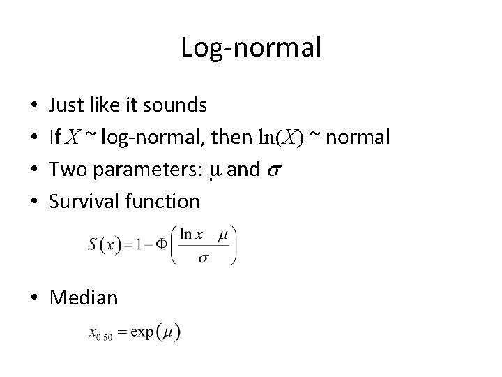
Log-normal • • Just like it sounds If X ~ log-normal, then ln(X) ~ normal Two parameters: m and s Survival function • Median
Log-normal • Log-normal can work well in medical applications (e. g. age of disease onset) • Hazard is hump-shaped • Critics think that decreasing hazard at later times is unrealistic
Log-logistic • If X ~ log-logistic, then ln(X) ~ logistic • Logistic is similar to normal, but the survival function is easier to work with • Hazard similar to Weibull, but more variable in shapes for hazard – Monotone decreasing – Hump-shaped
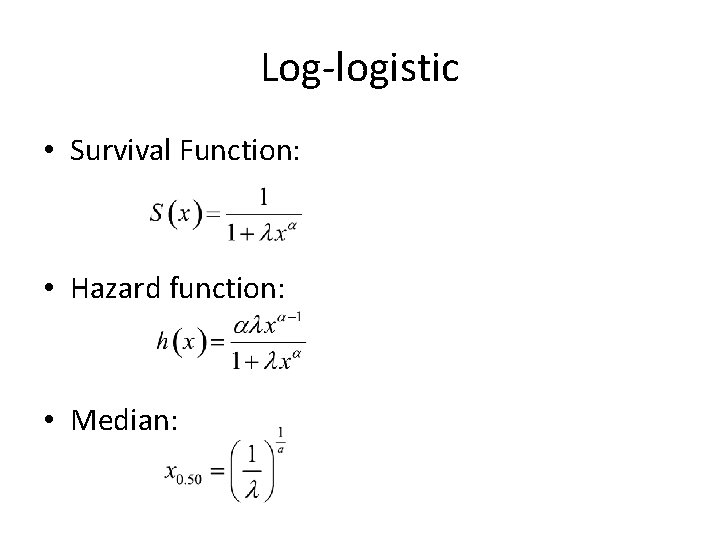
Log-logistic • Survival Function: • Hazard function: • Median:
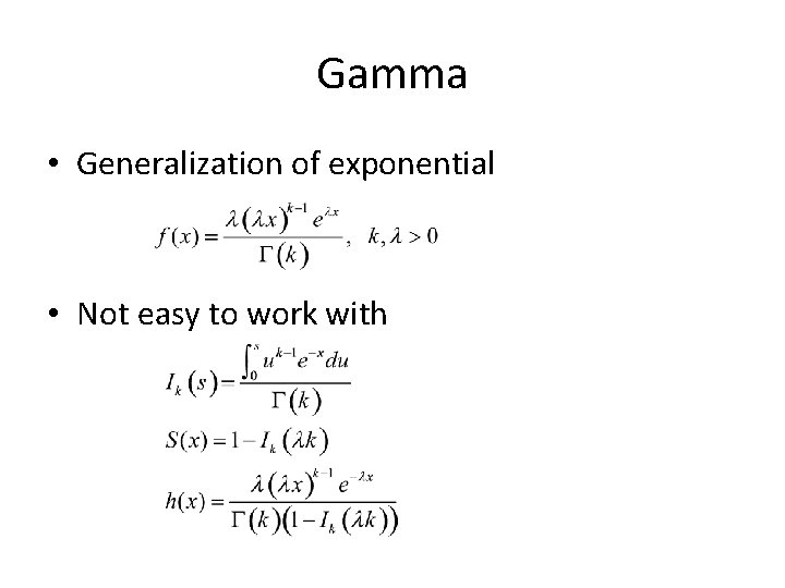
Gamma • Generalization of exponential • Not easy to work with
Cure Rate Distribution • Not in K & M • Assumption: fraction of individuals never fail • Violates assumption that S(∞) = 0 • Useful for clinical trials in which – A fraction of the patients are cured – Event my never occur (e. g. cancer relapse)
Cure Rate Example • 75% of women with early stage breast cancer are cured by treatment • Remaining 25% of women relapse – Assume exponential – l = 0. 05
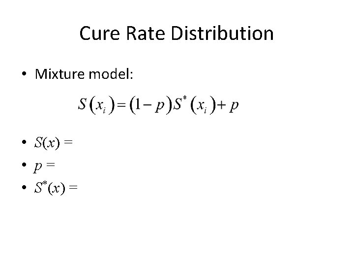
Cure Rate Distribution • Mixture model: • S(x) = • p= • S*(x) =
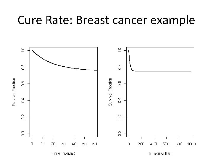
Cure Rate: Breast cancer example
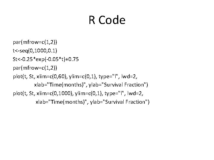
R Code par(mfrow=c(1, 2)) t<-seq(0, 1000, 0. 1) St<-0. 25*exp(-0. 05*t)+0. 75 par(mfrow=c(1, 2)) plot(t, St, xlim=c(0, 60), ylim=c(0, 1), type="l", lwd=2, xlab="Time(months)", ylab="Survival Fraction") plot(t, St, xlim=c(0, 1000), ylim=c(0, 1), type="l", lwd=2, xlab="Time(months)", ylab="Survival Fraction")
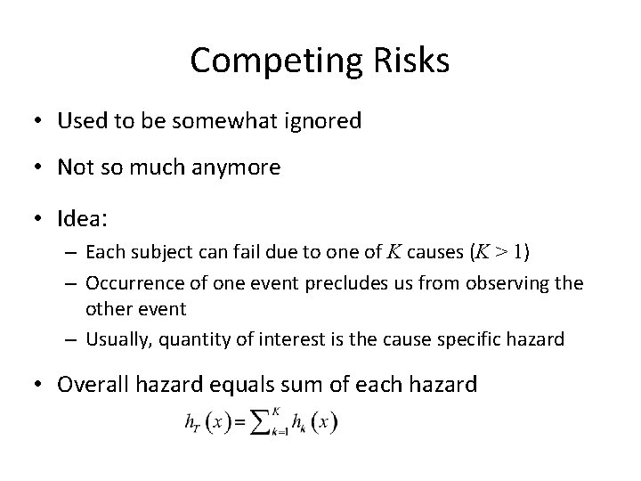
Competing Risks • Used to be somewhat ignored • Not so much anymore • Idea: – Each subject can fail due to one of K causes (K > 1) – Occurrence of one event precludes us from observing the other event – Usually, quantity of interest is the cause specific hazard • Overall hazard equals sum of each hazard
Example • An investigator is looking at graft rejection in kidney transplant patients • However… patients can also experience graft failure and death • Treat graft failure and graft rejection events as censored observations • Why is this a problem?
Assumptions • Dependence structure between the ‘potential’ failure times • Identifiability dilemma: – Can only observe one time person so not testable • We can not distinguish between independent and dependent competing risks
Useful Approaches • Want to account for other causes – Adjust the denominator • Compare rates of events – Use measures of probabilities • Crude: probability of event k allowing for all other risks • Net: probability of event k if it is the ONLY risk • Partial: probability of event k is one of a subset of risks acting in the population • See K & M for more details
- Slides: 64