Lecture 2 Divide and Conquer Basic Algorithm Design

Lecture 2: Divide and Conquer

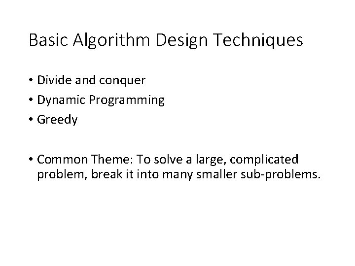
Basic Algorithm Design Techniques • Divide and conquer • Dynamic Programming • Greedy • Common Theme: To solve a large, complicated problem, break it into many smaller sub-problems.

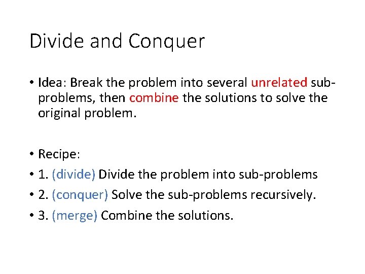
Divide and Conquer • Idea: Break the problem into several unrelated subproblems, then combine the solutions to solve the original problem. • Recipe: • 1. (divide) Divide the problem into sub-problems • 2. (conquer) Solve the sub-problems recursively. • 3. (merge) Combine the solutions.

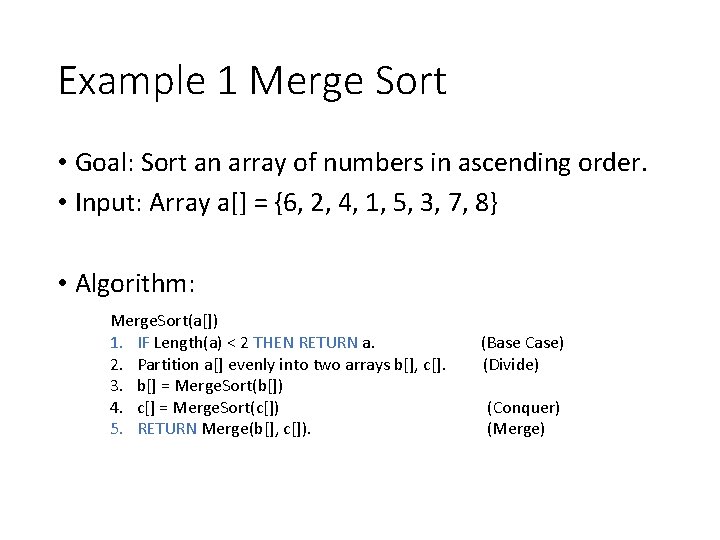
Example 1 Merge Sort • Goal: Sort an array of numbers in ascending order. • Input: Array a[] = {6, 2, 4, 1, 5, 3, 7, 8} • Algorithm: Merge. Sort(a[]) 1. IF Length(a) < 2 THEN RETURN a. 2. Partition a[] evenly into two arrays b[], c[]. 3. b[] = Merge. Sort(b[]) 4. c[] = Merge. Sort(c[]) 5. RETURN Merge(b[], c[]). (Base Case) (Divide) (Conquer) (Merge)

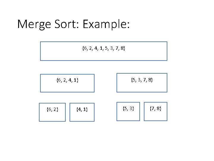
Merge Sort: Example: {6, 2, 4, 1, 5, 3, 7, 8} {1, 2, 3, 4, 5, 6, 7, 8} {6, 2, 4, 1} {1, 2, 4, 6} {6, 2} {2, 6} {4, 1} {1, 4} {5, 3, 7, 8} {3, 5, 7, 8} {5, 3} {3, 5} {7, 8}

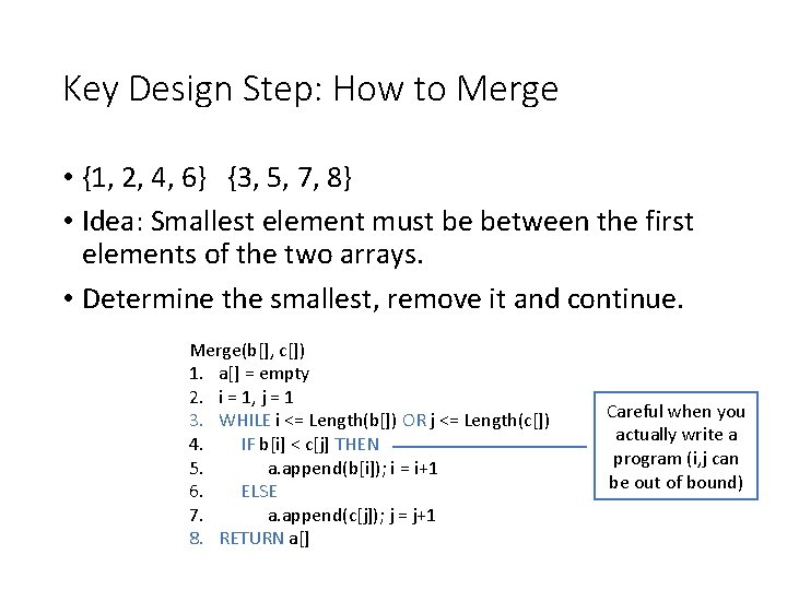
Key Design Step: How to Merge • {1, 2, 4, 6} {3, 5, 7, 8} • Idea: Smallest element must be between the first elements of the two arrays. • Determine the smallest, remove it and continue. Merge(b[], c[]) 1. a[] = empty 2. i = 1, j = 1 3. WHILE i <= Length(b[]) OR j <= Length(c[]) 4. IF b[i] < c[j] THEN 5. a. append(b[i]); i = i+1 6. ELSE 7. a. append(c[j]); j = j+1 8. RETURN a[] Careful when you actually write a program (i, j can be out of bound)

Example 2 Counting Inversions • Goal: Given array a[], count the number of pairs (i, j) such that i < j but a[i] > a[j]. • Input: Array a[] = {6, 2, 4, 1, 5, 3, 7, 8} • Answer = 9

Designing the algorithm • Recall Recipe: • 1. (divide) Divide the problem into sub-problems • 2. (conquer) Solve the sub-problems recursively. • 3. (merge) Combine the solutions.

Failed Attempt: • Partition a[] evenly to two arrays b[], c[]. • Count Inversions recursively. • Combine results • a[] = {6, 2, 4, 1, 5, 3, 7, 8}, 9 inversions b[] = {6, 2, 4, 1}, 5 inversions c[] = {5, 3, 7, 8}, 1 inversion • #inversion = #inversion in b + #inversion in c + #inversion between b[], c[] Can take O(n 2) time!

How to count inversions more efficiently? • b[] = {6, 2, 4, 1}, 5 inversions c[] = {5, 3, 7, 8}, 1 inversion • For each number in b, want to know how many numbers in c are smaller. 6: 2, 2: 0, 4: 1, 1: 0, result = 2+0+1+0 = 3. • Much easier if c[] is sorted! • Idea: Can sort the arrays when we are counting inversions.

Sort&Count(a[]) 1. IF Length(a) < 2 THEN RETURN (a[], 0). 2. Partition a[] evenly into two arrays b[], c[]. 3. (b[], count_b) = Sort&Count(b[]) 4. (c[], count_c) = Sort&Count(c[]) 5. (a[], count_bc) = Merge&Count(b[], c[]). 6. RETURN a[], count_b+count_c+count_bc. (Base Case) (Divide) (Conquer) (Merge)

Merge&Count • b[] = {1, 2, 4, 6} c[] = {3, 5, 7, 8} • {1, 2, 3, 4, 5, 6, 7, 8} • When 4 goes into the array, pointer in c[] is pointing at 5 (2 nd element), so 4 is larger than 1 element in c[]. • When 6 goes into the array, pointer in c[] is pointing at 7 (3 rd element), so 6 is larger than 2 elements in c[].

Merge&Count(b[], c[]) 1. a[] = empty 2. i = 1, j = 1 3. count = 0 4. WHILE i <= Length(b[]) OR j <= Length(c[]) 5. IF b[i] < c[j] THEN 6. a. append(b[i]); i = i+1 7. count = count + (j - 1) 8. ELSE 9. a. append(c[j]); j = j+1 10. RETURN a[], count The i-th element of a[] is smaller than c[j], but larger than c[1, 2, …, j-1]