Lecture 2 Digital Image Processing Sampling Quantization 1


. –")
) =")
 of interest to us: 1.")
 includes the effect of wavelength or")


= A sin(ft) + Q 3 unknowns, to solve in equation we need 3")


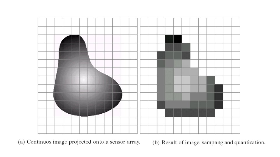
 a b c d Generating a digital image. (a) Continuous image.")


 – reading an image with different postfixes imresize() – resizing an image to")
![im=imread('obelix. jpg'); im=rgb 2 gray(imread('obelix. jpg')); im 1=imresize(im, [1024]); im 2=imresize(im 1, [1024]/2); im](https://slidetodoc.com/presentation_image_h2/b6659a24525954b3f572d47534fd5ed2/image-32.jpg "im=imread('obelix. jpg'); im=rgb 2 gray(imread('obelix. jpg')); im 1=imresize(im, [1024]); im 2=imresize(im 1, [1024]/2); im")

![generating figure of previous slide im=imread('obelix. jpg'); im=rgb 2 gray(imread('obelix. jpg')); im 1=imresize(im, [1024]);](https://slidetodoc.com/presentation_image_h2/b6659a24525954b3f572d47534fd5ed2/image-34.jpg "generating figure of previous slide im=imread('obelix. jpg'); im=rgb 2 gray(imread('obelix. jpg')); im 1=imresize(im, [1024]);")
![figure; subplot(2, 4, 1); imshow(im 1, []); subplot(2, 4, 2); imshow(im 2, []) subplot(2,](https://slidetodoc.com/presentation_image_h2/b6659a24525954b3f572d47534fd5ed2/image-35.jpg "figure; subplot(2, 4, 1); imshow(im 1, []); subplot(2, 4, 2); imshow(im 2, []) subplot(2,")


 has two vertical and two")
 are given")
 and N 4(P) are together known")


 y x (x-1, y-1) (x+1, y-1) (x-1, y)")

 (x+1, y-1) (x-1, y) p (x+1, y) (x-1,")
 (x+1, y-1) Diagonal neighbors of p: p ND(p)")


 to pixel q at (s,")


, (s, t) and")
 is defined as 2 2 2 1 0")
 is defined as 2 2 2 1 1")

- Slides: 59
Lecture # 2 Digital Image Processing Sampling & Quantization 1 st Semester 2019 -2020 Dr. Abdulhussein Mohsin Abdullah Computer Science Dept. , CS & IT College, Basrah Univ.
Elements of visual perception v Goal: help an observer interpret the content of an image v Developing a basic understanding of the visual process is important v Brief coverage of human visual perception follows – Emphasis on concepts that relate to subsequent material
Image Formation
image formation The amount of light reflected by an object in the physical world (3 d world) is pass through the lens of the camera and it becomes a 2 d signal.
For natural images we need a light source (λ: wavelength of the source). – E(x, y, z, λ): incident light on a point (x, y, z world coordinates of the point) Each point in the scene has a reflectivity function. – r(x, y, z, λ): reflectivity function Light reflects from a point and the reflected light is captured by an imaging device. • – c(x, y, z, λ) = E(x, y, z, λ) × r(x, y, z, λ): reflected light. • • • E(x, y, z, λ) c(x, y, z, λ) = E(x, y, z, λ) × r(x, y, z, λ) Camera (c(x, y, z, λ)) =
Inside the Camera - Projection Camera (c(x, y, z, λ)) =
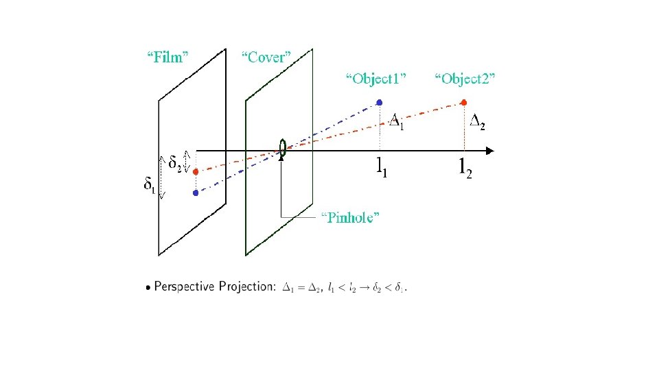
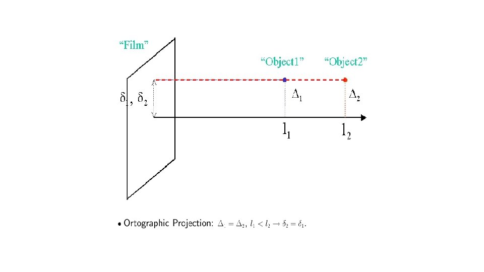
• There are two types of projections (P) of interest to us: 1. Perspective Projection – Objects closer to the capture device appear bigger. Most image formation situations can be considered to be under this category, including images taken by camera and the human eye. 2. Orthographic Projection – This is “unnatural”. Objects appear the same size regardless of their distance to the “capture device”. • Both types of projections can be represented via mathematical formulas. Orthographic projection is easier and is sometimes used as a mathematical convenience.
• The function f (x, y, λ) includes the effect of wavelength or frequency of the measured radiation. • Visible light has wavelengths, λ, from about 400 nm (blue) to 700 nm (red). • This will produce a single-band image, • where si(λ) is the sensitivity of the ith sensor, which defines the ith band. We often denote the N-band image by the vector • It is often the case that each of the bands is treated as a monochrome image.
Inside the Camera - Sensitivity
Sensitivity and Color
Summary
First Look at Sampling, Aliasing, Sampling and Aliasing
• What happens when you look at a textured object in a steep angle? image plane camera/eye check erboar d textu re
Aliasing • What happens when you look at a textured object in a steep angle? – Even though every ray corresponds to a distance of one pixel in the image, the world-space intervals get larger – At some point, we start missing the squares altogether – If we just take one point sample at the hit location, we get pretty much random results! CS-C 3100 Fall 2018 – Lehtinen
Aliasing – What Does it Look Like? Image: Xiaohu Zhang
q Most things in the real world are continuous, yet everything in a computer is discrete q The process of mapping a continuous function to a discrete one is called sampling q The process of mapping a continuous variable to a discrete one is called quantization q To represent or render an image using a computer, we must both sample and quantize
continuous value discrete value
Down-sampling
Aliasing can arise when you sample a continuous signal or image – occurs when your sampling rate is not high enough to capture the amount of detail in your image – Can give you the wrong signal/image—an alias – the sampling rate must be high enough to capture the highest frequency in the image To avoid aliasing: – sampling rate ≥ 2 * max frequency in the image • said another way: ≥ two samples per cycle – This minimum sampling rate is called the Nyquist rate
• The Amplitude is the height from the center line to the peak • The Phase Shift is how far the function is shifted horizontally / vertically from the usual position. • The Period goes from one peak to the next (or from any point to the next matching point): • The frequency of a trigonometric function is the number of cycles it completes in a given interval.
F(t)= A sin(ft) + Q 3 unknowns, to solve in equation we need 3 points. That is mean we need Amplitude Nyquist Rate = 2 f Frequency Phase 1 cycle in period time T
2 D example
Types of Image Sensors Single Sensor Line Sensor Array Sensor
y (intensity values) a b c d Generating a digital image. (a) Continuous image. (b) A scaling line from A to B in the continuous image, used to illustrate the concepts of sampling and quantization. (c) sampling and quantization. (d) Digital scan line.
0 0 0 75 75 75 128 128 255 255 75 75 75 200 200 255 255 200 128 128 200 255 200 200 128 128 255 200 200 75 75 175 175 225 225 75 75 75 100 175 100 100 225 75 75 100 75 75 75 35 35 35 0 0 0 35 35 35 75 75 100 100 200 200
Sampling
imread() – reading an image with different postfixes imresize() – resizing an image to any given size figure – opening a new graphical window subplot(#of row, # of col, location) – showing different plots/images in one graphical window imshow() – displaying an image Matlab
im=imread('obelix. jpg'); im=rgb 2 gray(imread('obelix. jpg')); im 1=imresize(im, [1024]); im 2=imresize(im 1, [1024]/2); im 3=imresize(im 1, [1024]/4); im 4=imresize(im 1, [1024]/8); im 5=imresize(im 1, [1024]/16); im 6=imresize(im 1, [1024]/32); 32 64 figure; imshow(im 1) figure; imshow(im 2) figure; imshow(im 3) figure; imshow(im 4) figure; imshow(im 5) 128 256 512 1024
Quantization 8 -bit 7 -bit 6 -bit 5 -bit 4 -bit 3 -bit 2 -bit 1 -bit
generating figure of previous slide im=imread('obelix. jpg'); im=rgb 2 gray(imread('obelix. jpg')); im 1=imresize(im, [1024]); im 2= gray 2 ind(im 1, 2^7); im 3= gray 2 ind(im 1, 2^6); im 4= gray 2 ind(im 1, 2^5); im 5= gray 2 ind(im 1, 2^4); im 6= gray 2 ind(im 1, 2^3); im 7= gray 2 ind(im 1, 2^2); im 8= gray 2 ind(im 1, 2^1);
figure; subplot(2, 4, 1); imshow(im 1, []); subplot(2, 4, 2); imshow(im 2, []) subplot(2, 4, 3); imshow(im 3, []); subplot(2, 4, 4); imshow(im 4, []) subplot(2, 4, 5); imshow(im 5, []); subplot(2, 4, 6); imshow(im 6, []) subplot(2, 4, 7); imshow(im 7, []); subplot(2, 4, 8); imshow(im 8, [])
Spatial and Intensity Resolution • Sampling is the principal factor defining the spatial resolution of an image, and quantization is the principal factor defining the intensity resolution. • Spatial resolution - number of rows and columns for example: 128 x 128, 256 by 256, etc. ; -->see Figs. 2. 19 and 2. 20 • Intensity resolution - number of gray levels for example: 8 bits, 16 bits, etc. ;
How to select the suitable size and pixel depth of images The word “suitable” is subjective: depending on “subject”. Low detail image Lena image Medium detail image High detail image Cameraman image To satisfy human mind 1. For images of the same size, the low detail image may need more pixel depth. 2. As an image size increase, fewer gray levels may be needed. (Images from Rafael C. Gonzalez and Richard E. Wood, Digital Image Processing, 2 nd Edition.
Neighbors of a Pixel • Any pixel p(x, y) has two vertical and two horizontal neighbors, given by (x+1, y), (x-1, y), (x, y+1), (x, y-1) • This set of pixels are called the 4 -neighbors of P, and is denoted by N 4(P). • Each of them are at a unit distance from P.
Neighbors of a Pixel • The four diagonal neighbors of p(x, y) are given by, (x+1, y+1), (x+1, y-1), (x-1, y+1), (x-1 , y-1) • This set is denoted by ND(P). • Each of them are at Euclidean distance of 1. 414 from P.
Neighbors of a Pixel • The points ND(P) and N 4(P) are together known as 8 -neighbors of the point P, denoted by N 8(P). • Some of the points in the N 4, ND and N 8 may fall outside image when P lies on the border of image.
Neighbors of a Pixel Neighbors of a pixel a. 4 -neighbors of a pixel p are its vertical and horizontal neighbors denoted by N 4(p) b. 8 -neighbors of a pixel p are its vertical horizontal and 4 diagonal neighbors denoted by N 8(p) p N 4(p) p N 8(p)
Neighbors of a Pixel ND N 4 P N 4 ND • N 4 - 4 -neighbors • ND - diagonal neighbors • N 8 - 8 -neighbors (N 4 U ND)
Basic Relationship of Pixels (0, 0) y x (x-1, y-1) (x+1, y-1) (x-1, y) (x+1, y) (x-1, y+1) (x+1, y+1) Conventional indexing method
Neighbors of a Pixel Neighborhood relation is used to tell adjacent pixels. It is useful for analyzing regions. 4 -neighbors of p: (x, y-1) (x-1, y) p (x+1, y) N 4(p) = (x, y+1) (x-1, y) (x+1, y) (x, y-1) (x, y+1) 4 -neighborhood relation considers only vertical and horizontal neighbors. Note: q Î N 4(p) implies p Î N 4(q)
Neighbors of a Pixel (x-1, y-1) (x+1, y-1) (x-1, y) p (x+1, y) (x-1, y+1) (x+1, y+1) 8 -neighbors of p: N 8(p) = (x-1, y-1) (x+1, y-1) (x-1, y) (x+1, y) (x-1, y+1) (x+1, y+1) 8 -neighborhood relation considers all neighbor pixels.
Neighbors of a Pixel (x-1, y-1) (x+1, y-1) Diagonal neighbors of p: p ND(p) = (x-1, y+1) (x+1, y+1) (x-1, y-1) (x+1, y-1) (x-1, y+1) (x+1, y+1) Diagonal -neighborhood relation considers only diagonal neighbor pixels.
Adjacency • Two pixels are connected if they are neighbors and their gray levels satisfy some specified criterion of similarity. • For example, in a binary image two pixels are connected if they are 4 -neighbors and have same value (0/1).
Connectivity is adapted from neighborhood relation. Two pixels are connected if they are in the same class (i. e. the same color or the same range of intensity) and they are neighbors of one another. Let V be set of gray levels values used to define adjacency. For p and q from the same class w 4 -connectivity: p and q are 4 -connected if q Î N 4(p) w 8 -connectivity: p and q are 8 -connected if q Î N 8(p) w mixed-connectivity (m-connectivity): p and q are m-connected if 1. q Î N 4(p) or 2. q Î ND(p) and N 4(p) Ç N 4(q) = Æ
Connectivity : To determine whether the pixels are adjacent in some sense. • Let V be the set of gray-level values used to define connectivity of the pixels p, q that have values from the set V are: a. 4 -connected, if q is in the set N 4(p) b. 8 -connected, if q is in the set N 8(p) c. m-connected, iff i. q is in N 4(p) or ii. q is in ND(p) and the set N 4 ( p) I N 4 (q) is empty V = {1, 2} 0 1 1 0 2 0 a. 0 0 1 0 1 1 0 2 0 0 0 1 b. c.
Adjacency/Connectivity 0 1 1 0 0 0 1 8 -adjacent m-adjacent
Adjacency A pixel p is adjacent to pixel q is they are connected. Two image subsets S 1 and S 2 are adjacent if some pixel in S 1 is adjacent to some pixel in S 2 S 1 S 2 We can define type of adjacency: 4 -adjacency, 8 -adjacency or m-adjacency depending on type of connectivity.
Path A path from pixel p at (x, y) to pixel q at (s, t) is a sequence of distinct pixels: (x 0, y 0), (x 1, y 1), (x 2, y 2), …, (xn, yn) such that (x 0, y 0) = (x, y) and (xn, yn) = (s, t) and (xi, yi) is adjacent to (xi-1, yi-1), i = 1, …, n • Here n is the length of the path. p q We can define type of path: 4 -path, 8 -path or m-path depending on type of adjacency.
Path 8 -path p q 8 -path from p to q results in some ambiguity m-path p q m-path from p to q solves this ambiguity
Regions and Boundaries • A subset R of pixels in an image is called a Region of the image if R is a connected set. • The boundary of the region R is the set of pixels in the region that have one or more neighbors that are not in R. • If R happens to be entire Image?
Distance For pixel p, q, and z with coordinates (x, y), (s, t) and (u, v), D is a distance function or metric if w D(p, q) ³ 0 (D(p, q) = 0 if and only if p = q) w D(p, q) = D(q, p) w D(p, z) £ D(p, q) + D(q, z) Example: Euclidean distance
Distance D 4 -distance (city-block distance) is defined as 2 2 2 1 0 1 2 2 2 Pixels with D 4(p) = 1 is 4 -neighbors of p.
Distance D 8 -distance (chessboard distance) is defined as 2 2 2 1 1 1 2 2 1 0 1 2 2 1 1 1 2 2 2 Pixels with D 8(p) = 1 is 8 -neighbors of p.
V ={0, 1} V ={1, 2} Find path 4 -, 8 -, m- q 3 1 2 1 0 2 1 2 1 1 1 0 1 2 P