Lecture 2 Basic LP Formulation MCCARL AND SPREEN

Lecture 2: Basic LP Formulation MCCARL AND SPREEN TEXT CH. 2 HTTP: //AGECON 2. TAMU. EDU/PEOPLE/FACUL T Y/MCCARL-BRUCE/BOOKS. HTM
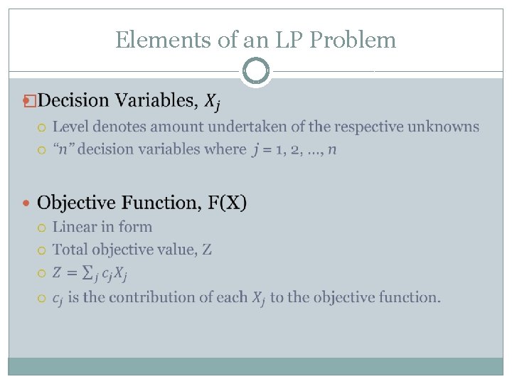
Elements of an LP Problem �
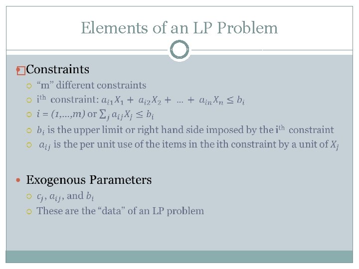
Elements of an LP Problem �
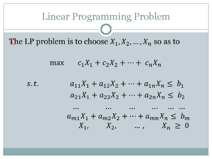
Linear Programming Problem �
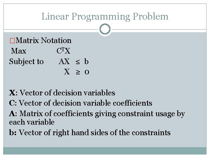
Linear Programming Problem �Matrix Notation Max CTX Subject to AX ≤ b X ≥ 0 X: Vector of decision variables C: Vector of decision variable coefficients A: Matrix of coefficients giving constraint usage by each variable b: Vector of right hand sides of the constraints
Elements of an LP Solution �
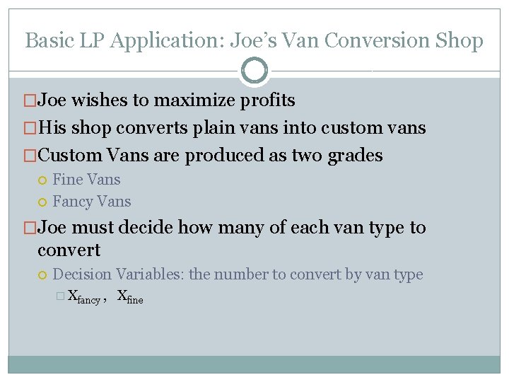
Basic LP Application: Joe’s Van Conversion Shop �Joe wishes to maximize profits �His shop converts plain vans into custom vans �Custom Vans are produced as two grades Fine Vans Fancy Vans �Joe must decide how many of each van type to convert Decision Variables: the number to convert by van type � Xfancy , Xfine
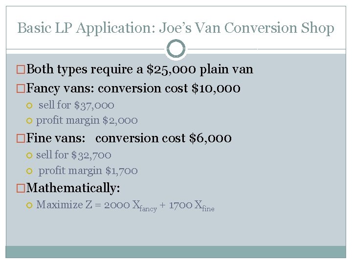
Basic LP Application: Joe’s Van Conversion Shop �Both types require a $25, 000 plain van �Fancy vans: conversion cost $10, 000 sell for $37, 000 profit margin $2, 000 �Fine vans: conversion cost $6, 000 sell for $32, 700 profit margin $1, 700 �Mathematically: Maximize Z = 2000 Xfancy + 1700 Xfine
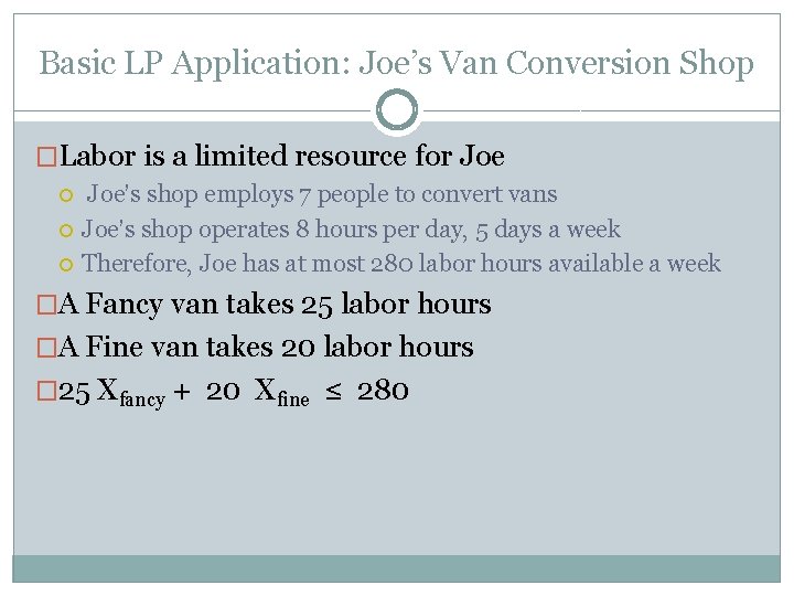
Basic LP Application: Joe’s Van Conversion Shop �Labor is a limited resource for Joe Joe’s shop employs 7 people to convert vans Joe’s shop operates 8 hours per day, 5 days a week Therefore, Joe has at most 280 labor hours available a week �A Fancy van takes 25 labor hours �A Fine van takes 20 labor hours � 25 Xfancy + 20 Xfine ≤ 280
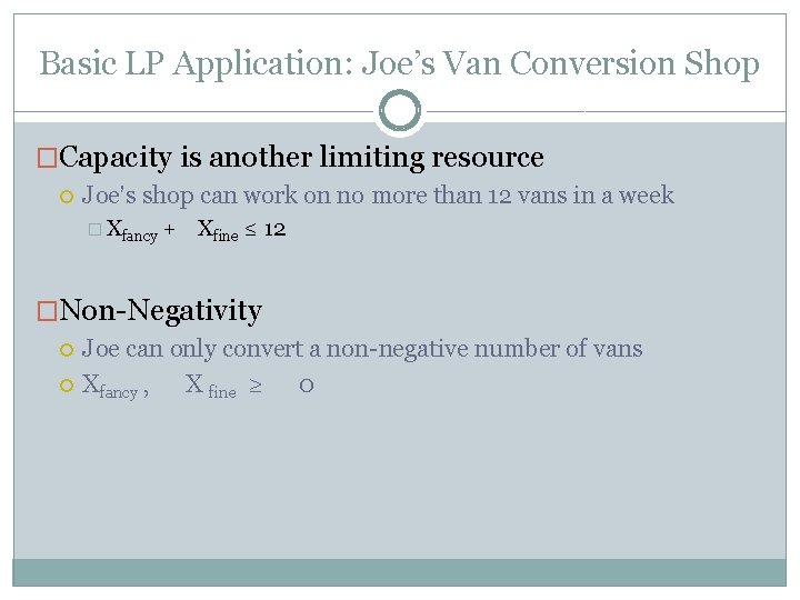
Basic LP Application: Joe’s Van Conversion Shop �Capacity is another limiting resource Joe’s shop can work on no more than 12 vans in a week � Xfancy + Xfine ≤ 12 �Non-Negativity Joe can only convert a non-negative number of vans Xfancy , X fine ≥ 0
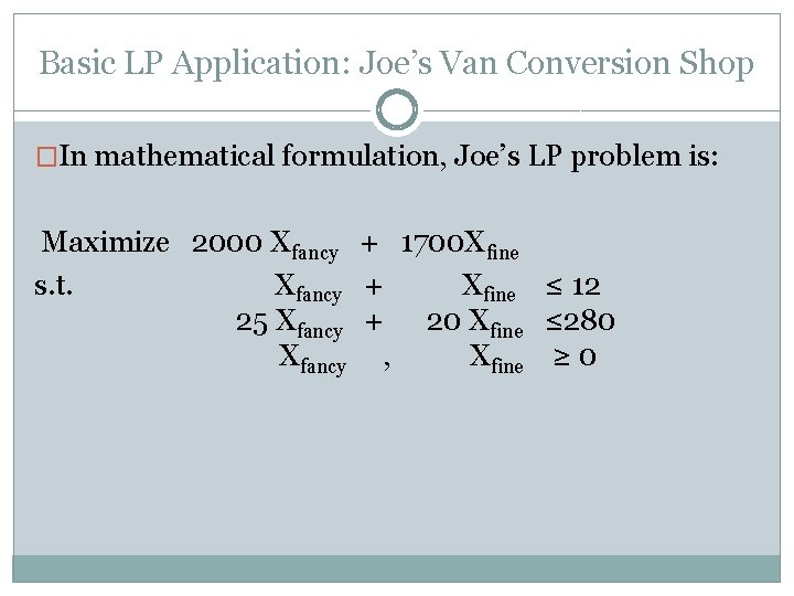
Basic LP Application: Joe’s Van Conversion Shop �In mathematical formulation, Joe’s LP problem is: Maximize 2000 Xfancy + 1700 Xfine s. t. Xfancy + Xfine ≤ 12 25 Xfancy + 20 Xfine ≤ 280 Xfancy , Xfine ≥ 0
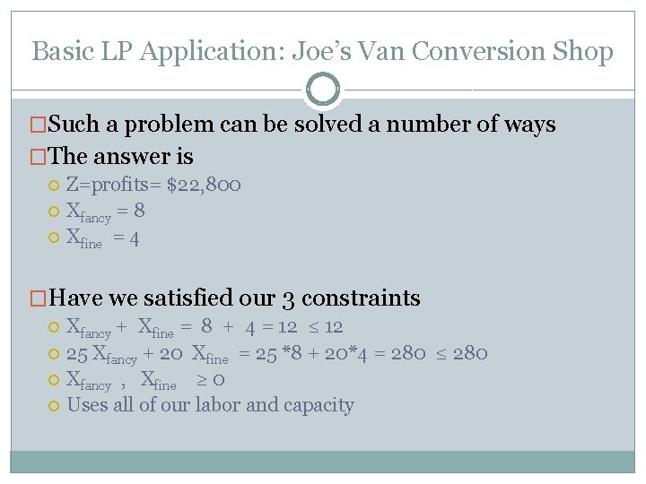
Basic LP Application: Joe’s Van Conversion Shop �Such a problem can be solved a number of ways �The answer is Z=profits= $22, 800 Xfancy = 8 Xfine = 4 �Have we satisfied our 3 constraints Xfancy + Xfine = 8 + 4 = 12 ≤ 12 25 Xfancy + 20 Xfine = 25 *8 + 20*4 = 280 ≤ 280 Xfancy , Xfine ≥ 0 Uses all of our labor and capacity
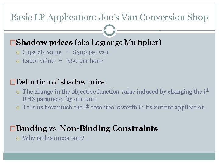
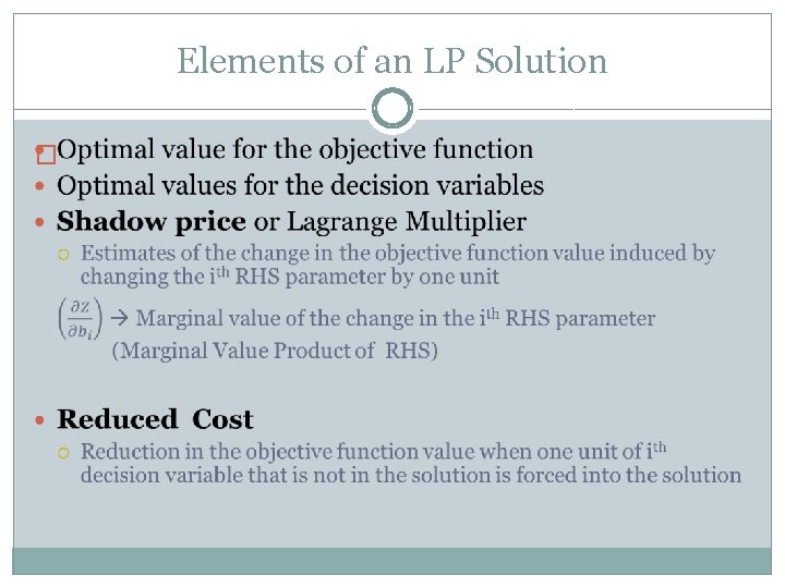
Basic LP Application: Joe’s Van Conversion Shop �Shadow prices (aka Lagrange Multiplier) Capacity value = $500 per van Labor value = $60 per hour �Definition of shadow price: The change in the objective function value induced by changing the ith RHS parameter by one unit Tells us how much the ith resource is worth in its current application �Binding vs. Non-Binding Constraints Why is this important?
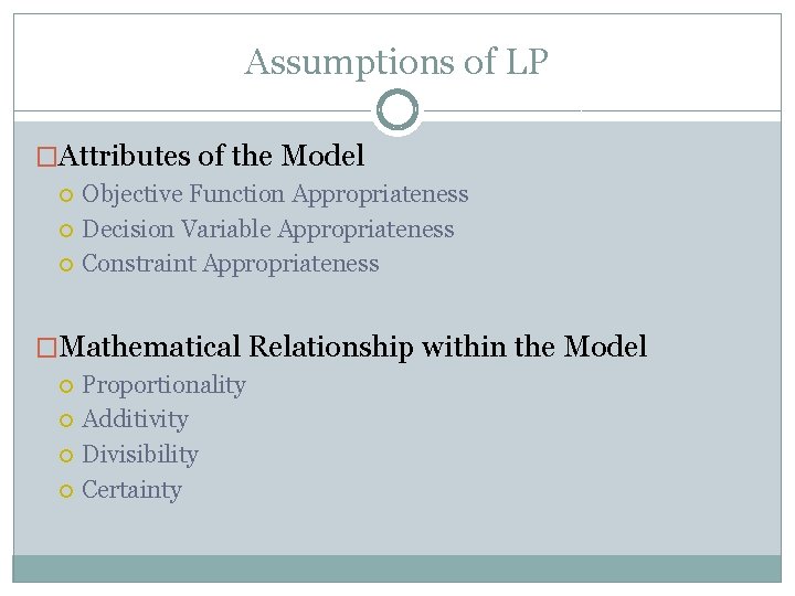
Assumptions of LP �Attributes of the Model Objective Function Appropriateness Decision Variable Appropriateness Constraint Appropriateness �Mathematical Relationship within the Model Proportionality Additivity Divisibility Certainty
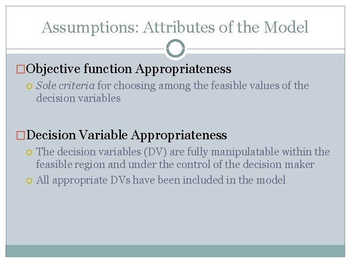
Assumptions: Attributes of the Model �Objective function Appropriateness Sole criteria for choosing among the feasible values of the decision variables �Decision Variable Appropriateness The decision variables (DV) are fully manipulatable within the feasible region and under the control of the decision maker All appropriate DVs have been included in the model
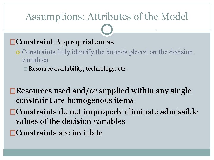
Assumptions: Attributes of the Model �Constraint Appropriateness Constraints fully identify the bounds placed on the decision variables � Resource availability, technology, etc. �Resources used and/or supplied within any single constraint are homogenous items �Constraints do not improperly eliminate admissible values of the decision variables �Constraints are inviolate
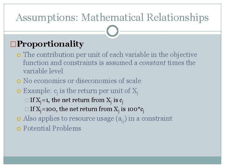
Assumptions: Mathematical Relationships �Proportionality The contribution per unit of each variable in the objective function and constraints is assumed a constant times the variable level No economics or diseconomies of scale Example: cj is the return per unit of Xj � If Xj=1, the net return from Xj is cj � If Xj=100, the net return from Xj is 100*cj Also applies to resource usage (aij) in a constraint Potential Problems
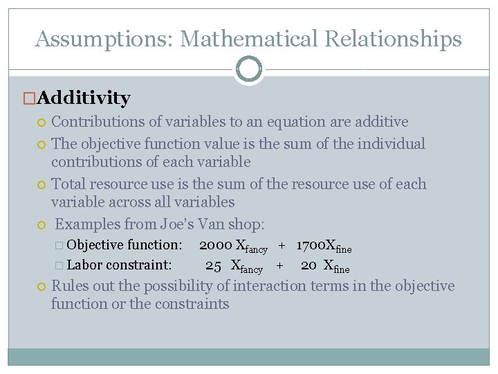
Assumptions: Mathematical Relationships �Additivity Contributions of variables to an equation are additive The objective function value is the sum of the individual contributions of each variable Total resource use is the sum of the resource use of each variable across all variables Examples from Joe’s Van shop: � Objective function: 2000 Xfancy + 1700 Xfine � Labor constraint: 25 Xfancy + 20 Xfine Rules out the possibility of interaction terms in the objective function or the constraints
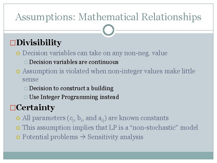
Assumptions: Mathematical Relationships �Divisibility Decision variables can take on any non-neg. value � Decision variables are continuous Assumption is violated when non-integer values make little sense � Decision to construct a building � Use Integer Programming instead �Certainty All parameters (cj, bi, and aij) are known constants This assumption implies that LP is a “non-stochastic” model Potential problems Sensitivity analysis
What We Know So Far… �Matrix and mathematical notations �Fundamental uses for LP �Basic model formulation �Key elements of an LP problem � 7 Assumptions of LP �Shadow prices and reduced costs
Where We are Going Next �Applying what we know to setting up and solving an LP problem In Excel (covered in first lab) Setting up the tableau (Overheads 3)
- Slides: 21