Lecture 2 5 Module 2 AVIATION TELECOMMUNICATION SYSTEMS

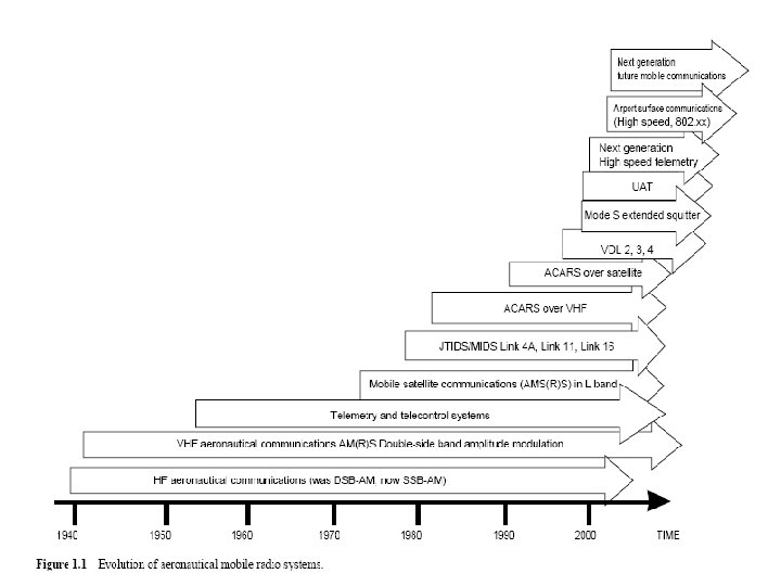
Lecture 2. 5. Module 2. AVIATION TELECOMMUNICATION SYSTEMS Topic 2. 5. Air and Ground Aviation communication Systems of Direct Visibility

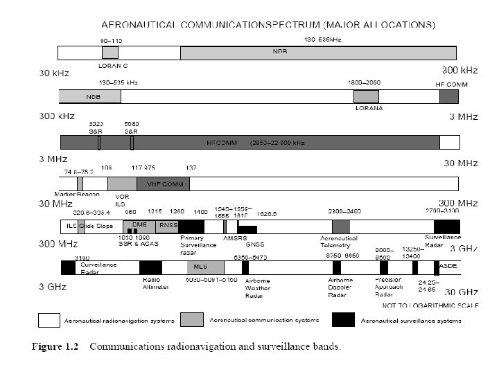
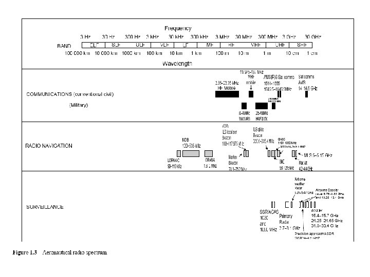
Radio Spectrum Used by Aviation Figures 1. 2 and 1. 3 depict the radio spectrum used by aeronautical communications today. The subject matter of most interest is probably: VHF (108– 137 MHz), L band (960– 1215 MHz), S band (2. 7– 3. 1 GHz) and C band (5. 000– 5. 250 GHz). Also shown in the figures are adjacent allocations to navigation and surveillance functions and some services.

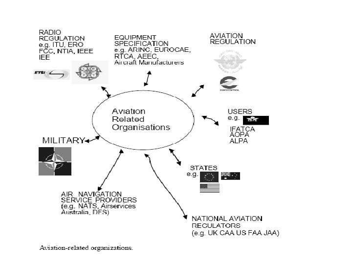
Example Standards Bodies and Professional Engineering Bodies There also a handful of standardizations bodies; some of them of relevance to this book include the following: - Aeronautical Radio Incorporated (ARINC) (www. arinc. com); - European Organisation for Civil Aviation Equipment (EUROCAE) (www. eurocae. org); - Radio Technical Commission for Aeronautics (RTCA) (www. rtca. org); - Airlines Electronic Engineering Committee (AEEC); - European Telecommunications Standards Institute (ETSI) (www. etsi. org); - SITA European Conference of Postal and Telecommunications Administrations (CEPT) - European Radiocommunications Office (ERO) (www. ero. dk); - International Telecommunications Union (ITU) (www. itu. org); - The Institute of Electrical and Electronic Engineers, Inc. (IEEE) (www. ieee. org); - The Institution of Engineering and Technology (IET) (www. iee. co. uk).

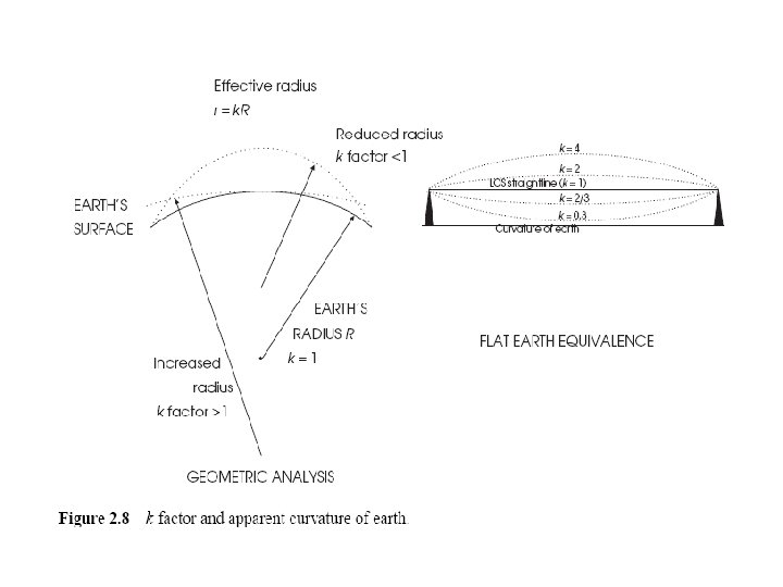
Earth Bulge Factor – k Factor In some instances, for designing radio links (particularly point–point terrestrial), it is found that radio waves do not propagate directly between two points with horizon grazing being the limiting factor as described above. They refract like light and generally tend to bend out from the earth but on occasion they bend towards the earth. This phenomenon can be described by incorporating what is called a k factor, which is used to change the apparent earth radius.

Conversely, k factors of greater than 1 would simulate the earth’s curvature decreasing, which is akin to rays diffracting upwards away from the earth and the horizon and subsequent LOS range of a link being pushed out. Statistical measurements have been collected by the ITU as to the proportion of the time k moves up and down for different frequencies and for different climate zones, and these have been incorporated in ITU recommendations (formerly CCIR recommendations). This consideration should be incorporated in design of radio links, particularly terrestrial point-topoint links or for low-flying scenarios. For LOS point-to-point links of high reliability, design k factors of 2/3 or even 0. 5 are sometimes taken. By substituting into the LOS horizon equation, this can be found to reduce the horizon by typically 10– 20 %. Apparent earth’s radius = k. R

Let’s consider the band used for mainstream civil aeronautical communications in the very high frequency band between 118 and 137 MHz.

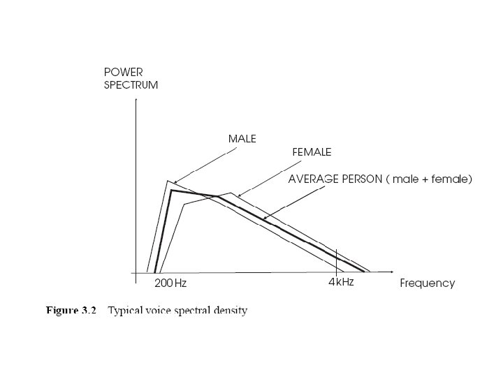
There were two criteria that were ultimately defining the bandwidth required by each of the radio frequency (RF) channels. Carrier frequency accuracy. The carrier frequency accuracy that could be achieved by both ground airborne transceiver equipment. This was becoming better all the time with technological improvement making it feasible to contain the modulated signal in a narrower band than the 200 k. Hz originally allocated. The actual bandwidth occupied by the DSB-AM spectrum. It should be noted that a typical unmodulated voice signal shows a spectral density with most of its power components above 200 Hz and below 4 k. Hz (Figure 3. 2).

So (today) it is possible to accurately re-create a voice signal by demodulating a signal with the carrier plus all the components band limited ± 4 k. Hz. (In comparison, for the music even CD quality is only ± 8 k. Hz. ) If a DSB-AM signal is created by modulating a carrier with a voice-limited signal to± 4 k. Hz, the modulated spectra will similarly be limited to ± 4 k. Hz about the carrier.

Channel Splitting Taking both the factors, channel frequency accuracy and the actual bandwidth occupied by the DSB-AM spectrum, into account it is possible to reduce the channel spacing and hence to increase the amount of channels available in the given spectrum.

In the 1950 s, – 100 k. Hz channel spacing was first introduced, which doubled the capacity to 140 available channels. In addition WRC 1959 further extended the band allocated for AM(R)S to 118– 136 MHz; this meant 180 channels at 100 k. Hz were achievable. In the 1960 s, this methodology was extended further, with 50 k. Hz channel spacing, and this doubled the capacity again to 360 channels at 50 k. Hz. In 1972, – 25 k. Hz channel spacing was introduced and this doubled the capacity again to a theoretical 720 channels. This alone was not enough to curb demand in 1979, WRC extended the AM(R)S allocation in the VHF band further to 117. 975– 137. 000 MHz, which is where it is today with a theoretical 760 channels at 25 k. Hz achievable. A further reason for the channel splitting approach was backward compatibility between old and new radio systems.

Today and 8. 33 k. Hz Channelization In 1996 again, driven by an increase in air traffic and consequently demand on VHF channels, a further channel split to 8. 33 k. Hz was proposed in Europe only. This gives a theoretical 2280 channels achievable. The choice of 8. 33 k. Hz was chosen as it was the minimum practical size to support DSB-AM modulation (if the ± 4 k. Hz voice limiting is applied as discussed above, a modulated channelization of 8 k. Hz can be obtained), and it theoretically provided a threefold increase in voice channel capacity. Further band limiting voice below 4 k. Hz would mean degradation in voice quality. So despite some interests saying it could be further channel split past 8. 33 k. Hz, this is likely to be the last realization of channel splitting and the end of the road for the DSB-AM technology.

Also it is unfortunate to see that aviation interests have fragmented into different regional policies, with Europe backing the 8. 33 k. Hz deployment and North America backing the seemingly oppositional VDL 3 solution (using 25 k. Hz channelization) rather than one international system deployed by all. This complicates equipage issues and future options, as will be seen later.

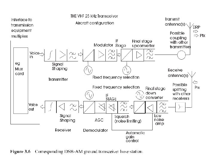
DSB-AM Transceiver at a System Level The system diagram is shown below and is applicable for 200, 100, 50, 25 and 8. 33 k. Hz channel working. It should be noted that modern receiver design may bypass the two-stage intermediate frequency process (as is defined in ICAO) and do it in a single voice frequency to radio frequency stage, or in some of the latest cutting-edge transceivers described later, the synthesis can even be carried out in a software on a modern processor using a fast sample period (multiple of the basic carrier rate) instead of the traditional crystal filter resonant circuits with harmonic generation synthesis.

The difference between the channelization being used will be reflected in the band-limiting filter at the end of the signal-shaping stage. Here the upper bandwidth cut -off of this filter must by definition be a maximum of half of the channel spacing. So at 25 k. Hz, it must be 12. 5 k. Hz and for 8. 33 k. Hz it must be 4. 165 k. Hz in its ideal form (4 k. Hz is used in practice). Similarly the corresponding receiver should have a matching low-pass filter as per above in its signalshaping circuitry dependent on the channelization being used. It will also be reflected in the thumbwheel dial selector used in the cockpit, which selects the channel frequency. On the ground the base station is usually fixed frequency working.

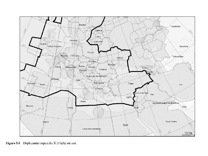
As previously pointed out, the majority of the voice power spectrum is contained below 4 k. Hz, so for the 8. 33 k. Hz system the voice signal can be reconstructed with most of the information being retained and just a minor degradation in quality to what was sent. Operationally the degradation with 8. 33 k. Hz is almost negligible to all but the most trained ear and as such it has been operationally accepted by all the regions shown in the map in Figure 3. 4.

Also because of this voice power spectrum, it means that an 8. 33 k. Hz radio is capable of receiving signals sent by 200, 100, 50 and 25 k. Hz working. Indeed this ‘backward compatibility’ of DSB-AM has been a key feature in its evolution. Similarly a 25 k. Hz radio would be able to receive an 8. 33 -k. Hz channel signal, provided it was tuned to the same carrier frequency.

System Design Features of AM(R)S DSB-AM System

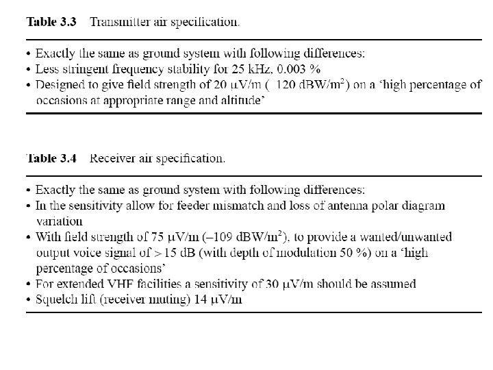
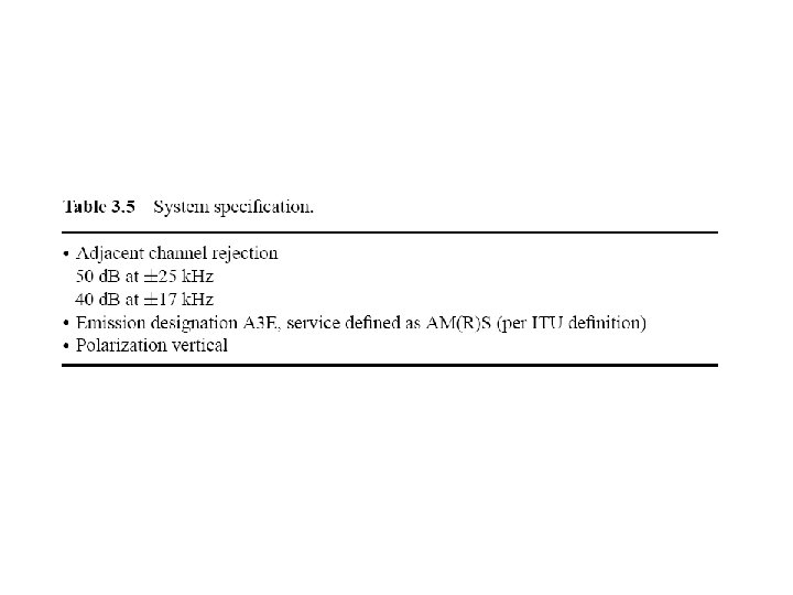
ICAO SARP’s Chapter 2 (Tables 3. 1– 3. 5).

Dimensioning a Mobile Communications System–The Three Cs A concept called the three Cs: These stand for coverage, capacity and ‘cwality’. In summary these are three determining criteria for any mobile communication system. This can be applied to the aeronautical mobile scenario.

Coverage This is the service area of a generic mobile system. Generically it could be split into typical rural, sub-urban or urban coverage areas, or in aeronautical equivalent terms as long distance en route coverage, terminal maneuvering area (TMA) coverage or local airport coverage.

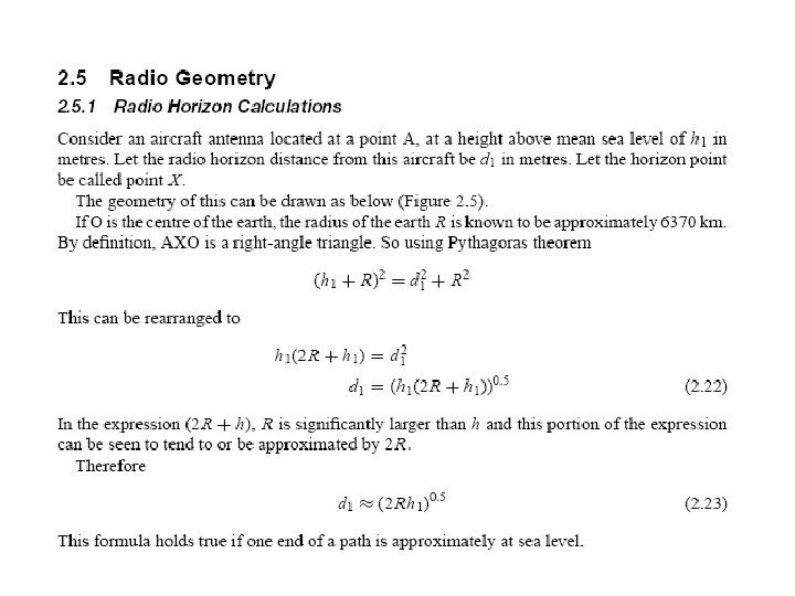
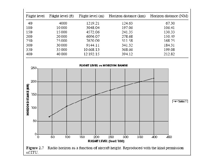
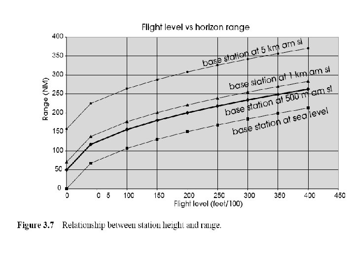
There is a relationship between height of the transmitting and receiving antennas (or flight level in the case of the airborne transceiver) and line-ofsight (LOS) distance or radius of coverage (Figure 3. 7). In general terms, the LOS distance can be considered as the limiting factor for long-distance VHF communications. (Over the horizon, the obstructed radio path sees dramatic increase in the attenuation; thus the effective usable coverage boundary is usually close to the horizon). This is applicable for the en route phases of flight and the upper airspace.

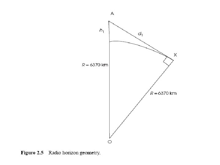
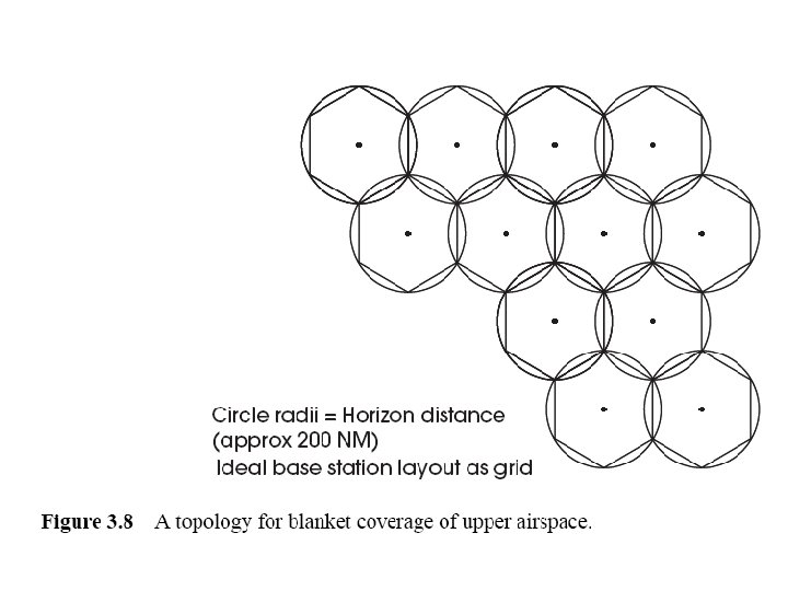
For upper airspace, a LOS link can be assumed to be ultimately limited by horizon and link budget (some further consideration should be given in mountainous areas or overseas). A conservative k factor is that of 2/3, allowing for refraction towards the earth. It generally gives a good conservative estimate to which horizon communications can be established and maintained for a very-high availability factor (>99. 9 %) (Figure 3. 8).

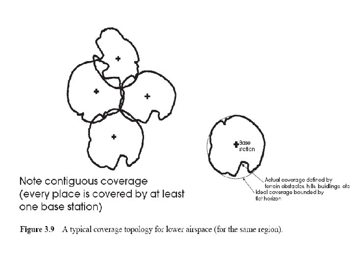
For ground links and low-airspace links, careful attention should be given to terrain, building clutter and any other likely obstructions, leading to links usually not being direct LOS links. Link budget design tools fitted with terrain and building geographical/topographical information should be used if available (Figure 3. 9).