Lecture 19 Word Sense Disambiguation CS 4705 Overview

Lecture 19 Word Sense Disambiguation CS 4705

Overview • Selectional restriction based approaches • Robust techniques – Machine Learning • Supervised • Unsupervised – Dictionary-based techniques

Disambiguation via Selectional Restrictions • Eliminates ambiguity by eliminating ill-formed semantic representations much as syntactic parsing eliminates ill-formed syntactic analyses – Different verbs select for different thematic roles wash the dishes (takes washable-thing as patient) serve delicious dishes (takes food-type as patient) • Method: rule-to-rule syntactico-semantic analysis – Semantic attachment rules are applied as sentences are syntactically parsed – Selectional restriction violation: no parse

• Requires: – Selectional restrictions for each sense of each predicate – Hierarchical type information about each argument (a la Word. Net) • Limitations: – Sometimes not sufficiently constraining to disambiguate (Which dishes do you like? ) – Violations that are intentional (Eat dirt, worm!) – Metaphor and metonymy

Selectional Restrictions as Preferences • Resnik ‘ 97, ‘ 98’s selectional association: – Probabilistic measure of strength of association between predicate and class dominating argument – Derive predicate/argument relations from tagged corpus – Derive hyponymy relations from Word. Net – Selects sense with highest selectional association between an ancestor and predicate (44% correct) Brian ate the dish. • WN: dish is a kind of crockery and a kind of food • tagged corpus counts: ate/<crockery> vs. ate/<food>

Machine Learning Approaches • Learn a classifier to assign one of possible word senses for each word – Acquire knowledge from labeled or unlabeled corpus – Human intervention only in labeling corpus and selecting set of features to use in training • Input: feature vectors – Target (dependent variable) – Context (set of independent variables) • Output: classification rules for unseen text

Input Features for WDS • POS tags of target and neighbors • Surrounding context words (stemmed or not) • Partial parsing to identify thematic/grammatical roles and relations • Collocational information: – How likely are target and left/right neighbor to co-occur Is the bass fresh today? [w-2, w-2/pos, w-1, w-/pos, w+1/pos, w+2/pos… [is, V, the, DET, fresh, RB, today, N. . .

• Co-occurrence of neighboring words – How often does sea or words with root sea (e. g. seashore, seafood, seafaring) occur in a window of size N – How choose? • M most frequent content words occurring within window of M in training data

Supervised Learning • Training and test sets with words labeled as to correct sense (It was the biggest [fish: bass] I’ve seen. ) – Obtain independent vars automatically (POS, cooccurrence information, etc. ) – Run classifier on training data – Test on test data – Result: Classifier for use on unlabeled data

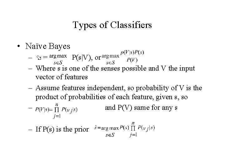
Types of Classifiers • Naïve Bayes – = P(s|V), or – Where s is one of the senses possible and V the input vector of features – Assume features independent, so probability of V is the product of probabilities of each feature, given s, so – and P(V) same for any s – If P(s) is the prior

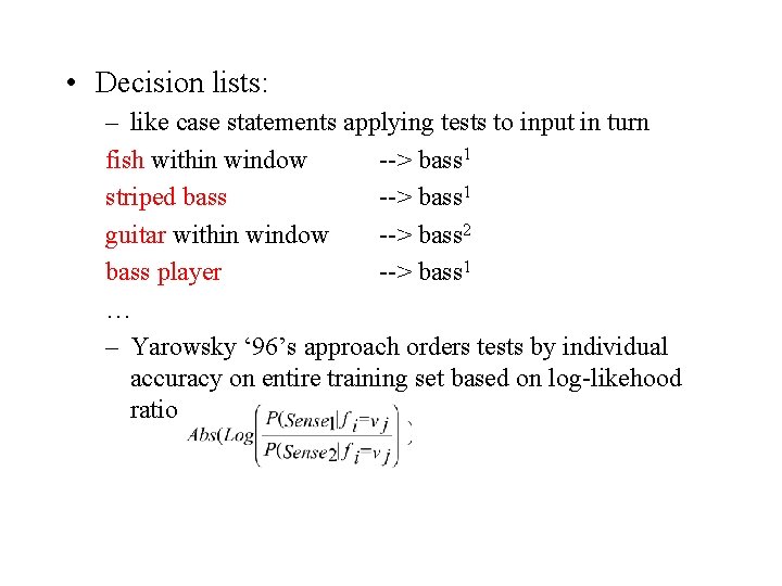
• Decision lists: – like case statements applying tests to input in turn fish within window --> bass 1 striped bass --> bass 1 guitar within window --> bass 2 bass player --> bass 1 … – Yarowsky ‘ 96’s approach orders tests by individual accuracy on entire training set based on log-likehood ratio

• Bootstrapping I – Start with a few labeled instances of target item as seeds to train initial classifier, C – Use high confidence classifications of C on unlabeled data as training data – Iterate • Bootstrapping II – Start with sentences containing words strongly associated with each sense (e. g. sea and music for bass), either intuitively or from corpus or from dictionary entries – One Sense per Discourse hypothesis

Unsupervised Learning • Cluster automatically derived feature vectors to ‘discover’ word senses using some similarity metric – Represent each cluster as average of feature vectors it contains – Label clusters by hand with known senses – Classify unseen instances by proximity to these known and labeled clusters • Evaluation problem – What are the ‘right’ senses?

– Cluster impurity – How do you know how many clusters to create? – Some clusters may not map to ‘known’ senses

Dictionary Approaches • Problem of scale for all ML approaches – Build a classifier for each sense ambiguity • Machine readable dictionaries (Lesk ‘ 86) – Retrieve all definitions of content words in context of target – Compare for overlap with sense definitions of target – Choose sense with most overlap • Limitations – Entries are short --> expand entries to ‘related’ words using subject codes