Lecture 18 Varimax Factors and Empircal Orthogonal Functions

Lecture 18 Varimax Factors and Empircal Orthogonal Functions

Syllabus Lecture 01 Lecture 02 Lecture 03 Lecture 04 Lecture 05 Lecture 06 Lecture 07 Lecture 08 Lecture 09 Lecture 10 Lecture 11 Lecture 12 Lecture 13 Lecture 14 Lecture 15 Lecture 16 Lecture 17 Lecture 18 Lecture 19 Lecture 20 Lecture 21 Lecture 22 Lecture 23 Lecture 24 Describing Inverse Problems Probability and Measurement Error, Part 1 Probability and Measurement Error, Part 2 The L 2 Norm and Simple Least Squares A Priori Information and Weighted Least Squared Resolution and Generalized Inverses Backus-Gilbert Inverse and the Trade Off of Resolution and Variance The Principle of Maximum Likelihood Inexact Theories Nonuniqueness and Localized Averages Vector Spaces and Singular Value Decomposition Equality and Inequality Constraints L 1 , L∞ Norm Problems and Linear Programming Nonlinear Problems: Grid and Monte Carlo Searches Nonlinear Problems: Newton’s Method Nonlinear Problems: Simulated Annealing and Bootstrap Confidence Intervals Factor Analysis Varimax Factors, Empircal Orthogonal Functions Backus-Gilbert Theory for Continuous Problems; Radon’s Problem Linear Operators and Their Adjoints Fréchet Derivatives Exemplary Inverse Problems, incl. Filter Design Exemplary Inverse Problems, incl. Earthquake Location Exemplary Inverse Problems, incl. Vibrational Problems

Purpose of the Lecture Choose Factors Satisfying A Priori Information of Spikiness (varimax factors) Use Factor Analysis to Detect Patterns in data (EOF’s)

Part 1: Creating Spiky Factors

can we find “better” factors that those returned by svd() ?

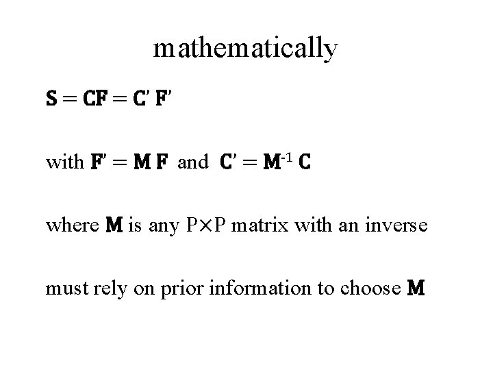
mathematically S = CF = C’ F’ with F’ = M F and C’ = M-1 C where M is any P×P matrix with an inverse must rely on prior information to choose M

one possible type of prior information factors should contain mainly just a few elements

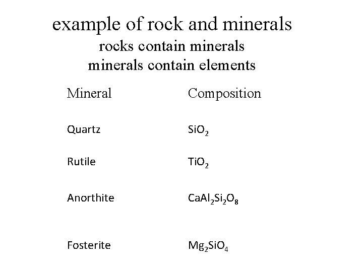
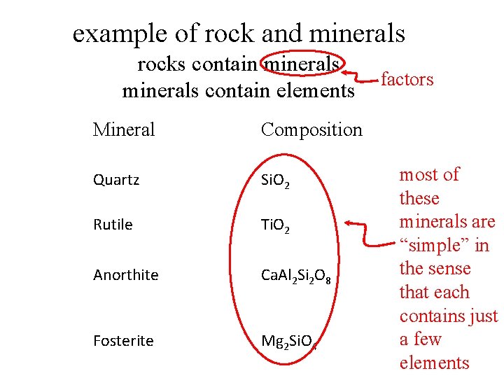
example of rock and minerals rocks contain minerals contain elements Mineral Composition Quartz Si. O 2 Rutile Ti. O 2 Anorthite Ca. Al 2 Si 2 O 8 Fosterite Mg 2 Si. O 4

example of rock and minerals rocks contain minerals contain elements Mineral Composition Quartz Si. O 2 Rutile Ti. O 2 Anorthite Ca. Al 2 Si 2 O 8 Fosterite Mg 2 Si. O 4 factors most of these minerals are “simple” in the sense that each contains just a few elements

spiky factors containing mostly just a few elements

How to quantify spikiness?

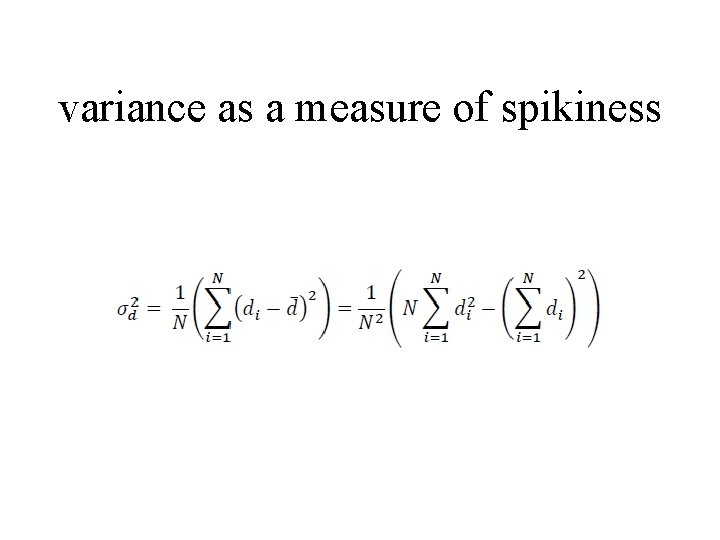
variance as a measure of spikiness

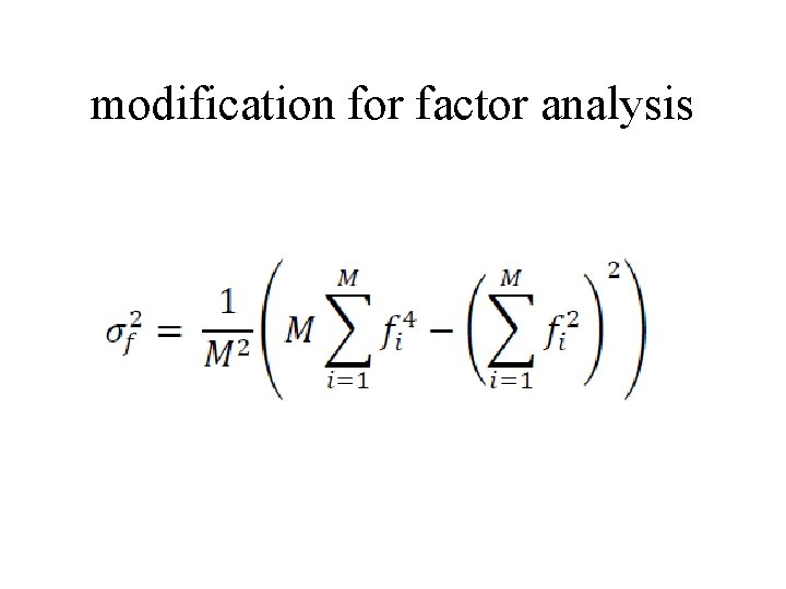
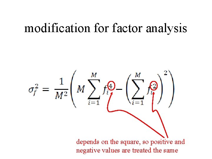
modification for factor analysis

modification for factor analysis depends on the square, so positive and negative values are treated the same

f(1)= [1, 0, 1, 0]T is much spikier than f(2)= [1, 1, 1, 1]T

f(2)=[1, 1, 1, 1]T is just as spiky as f(3)= [1, -1, -1, 1]T

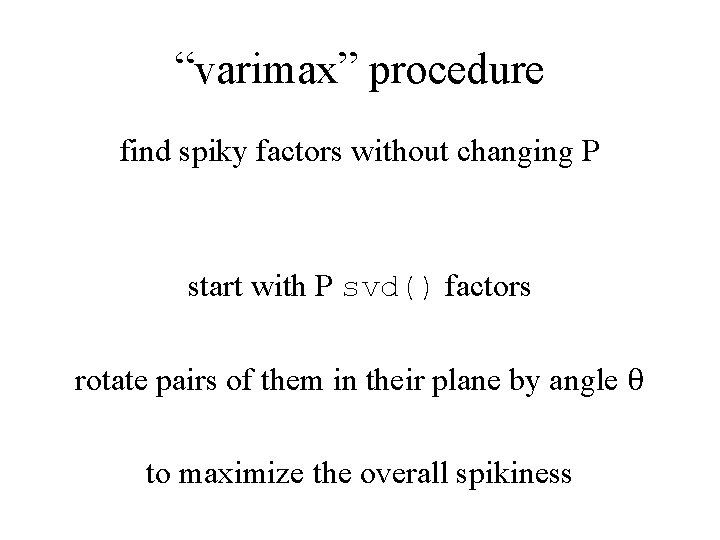
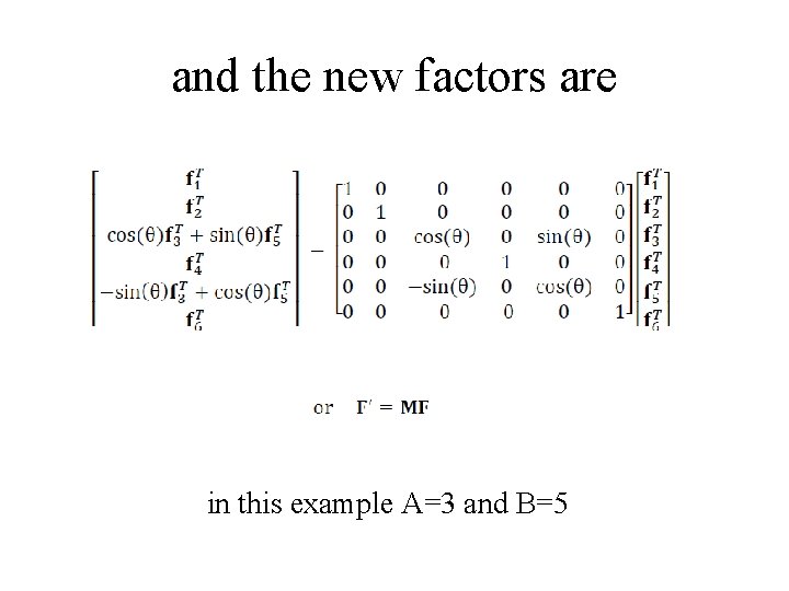
“varimax” procedure find spiky factors without changing P start with P svd() factors rotate pairs of them in their plane by angle θ to maximize the overall spikiness

f’A f. B f’B q f. A

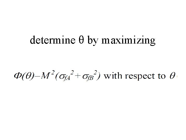
determine θ by maximizing

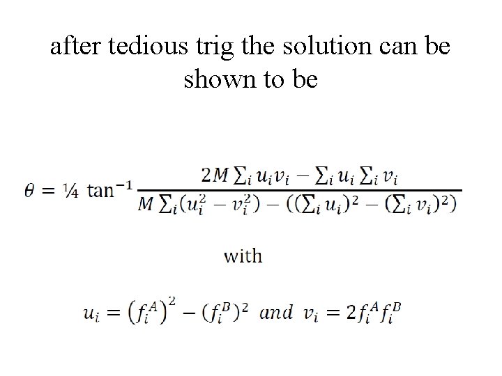
after tedious trig the solution can be shown to be

and the new factors are in this example A=3 and B=5

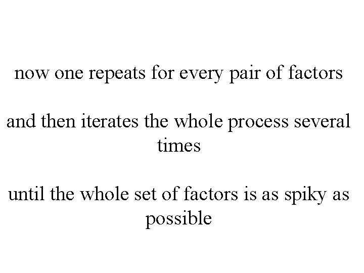
now one repeats for every pair of factors and then iterates the whole process several times until the whole set of factors is as spiky as possible

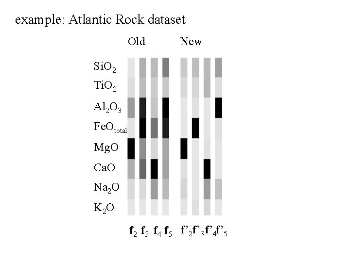
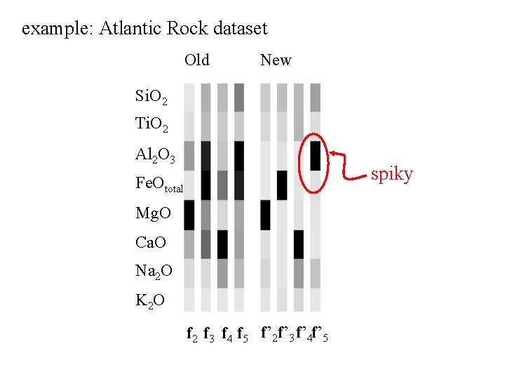
example: Atlantic Rock dataset Old New Si. O 2 Ti. O 2 Al 2 O 3 Fe. Ototal Mg. O Ca. O Na 2 O K 2 O f 2 f 3 f 4 f 5 f’ 2 f’ 3 f’ 4 f’ 5

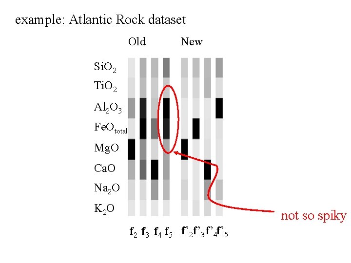
example: Atlantic Rock dataset Old New Si. O 2 Ti. O 2 Al 2 O 3 Fe. Ototal Mg. O Ca. O Na 2 O K 2 O not so spiky f 2 f 3 f 4 f 5 f’ 2 f’ 3 f’ 4 f’ 5

example: Atlantic Rock dataset Old New Si. O 2 Ti. O 2 Al 2 O 3 spiky Fe. Ototal Mg. O Ca. O Na 2 O K 2 O f 2 f 3 f 4 f 5 f’ 2 f’ 3 f’ 4 f’ 5

Part 2: Empirical Orthogonal Functions

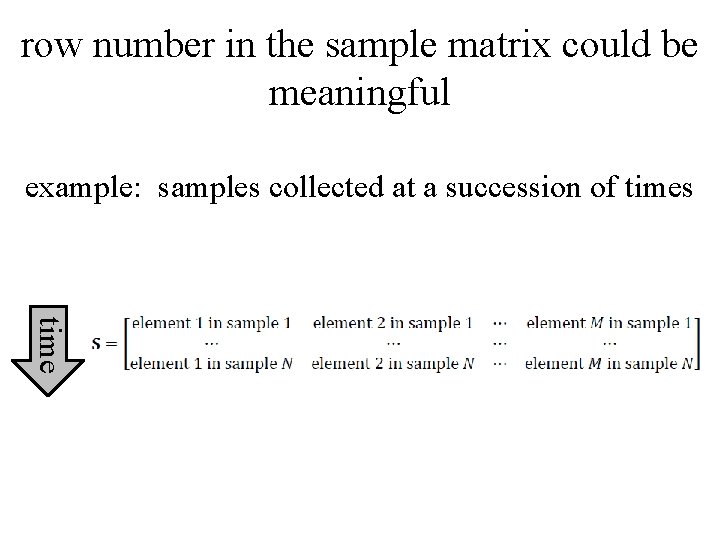
row number in the sample matrix could be meaningful example: samples collected at a succession of times time

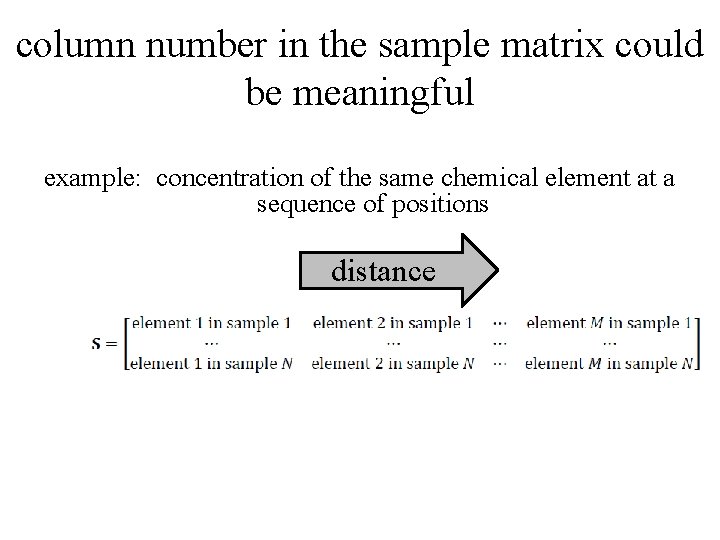
column number in the sample matrix could be meaningful example: concentration of the same chemical element at a sequence of positions distance

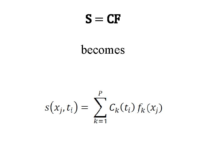
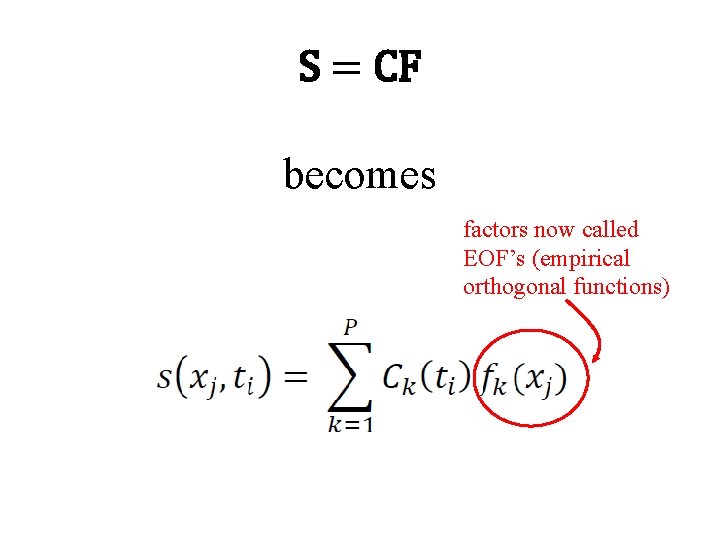
S = CF becomes

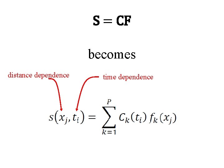
S = CF becomes distance dependence time dependence

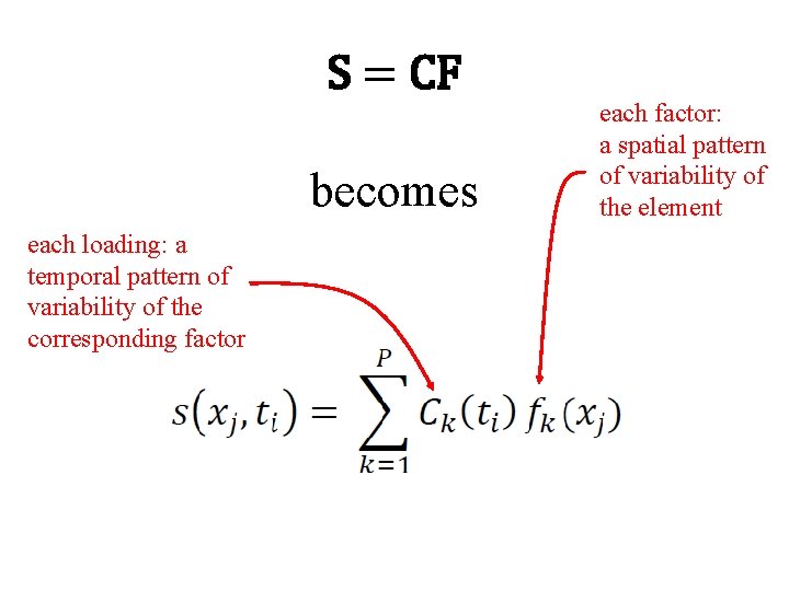
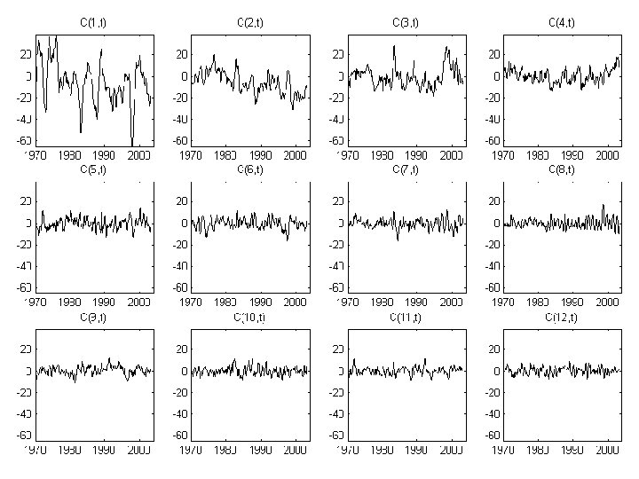
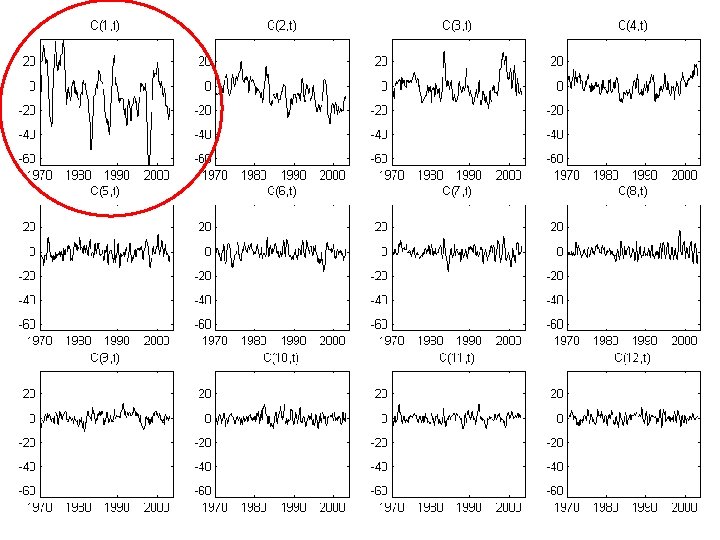
S = CF becomes each loading: a temporal pattern of variability of the corresponding factor each factor: a spatial pattern of variability of the element

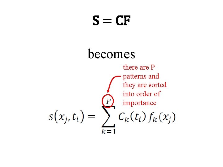
S = CF becomes there are P patterns and they are sorted into order of importance

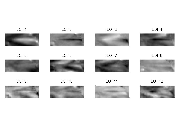
S = CF becomes factors now called EOF’s (empirical orthogonal functions)

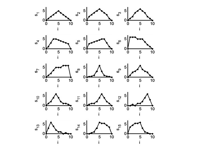
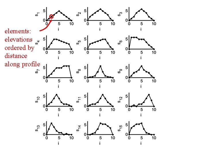
example 1 hypothetical mountain profiles what are the most important spatial patterns that characterize mountain profiles

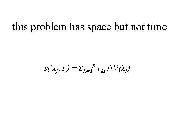
this problem has space but not time p s( xj , i ) = Σk=1 cki f (k)(xj)

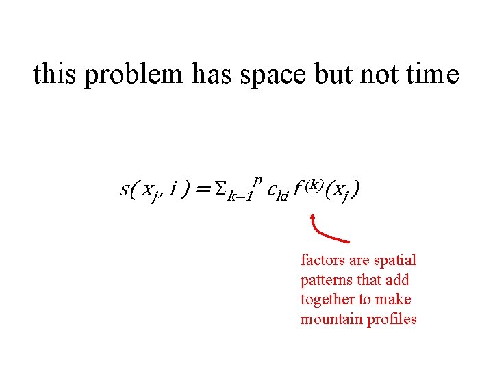
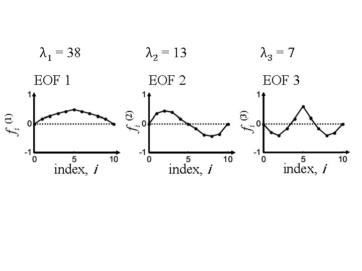
this problem has space but not time p s( xj , i ) = Σk=1 cki f (k)(xj ) factors are spatial patterns that add together to make mountain profiles

elements: elevations ordered by distance along profile

λ 1 = 38 λ 3 = 7 EOF 2 EOF 3 index, i fi (3) fi (1) fi (2) EOF 1 λ 2 = 13 index, i

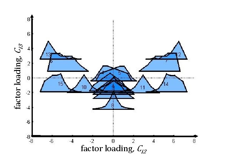
factor loading, Ci 3 factor loading, Ci 2

example 2 spatial-temporal patterns (synthetic data)

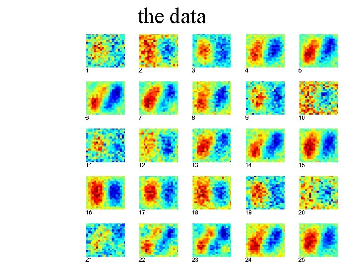
the data

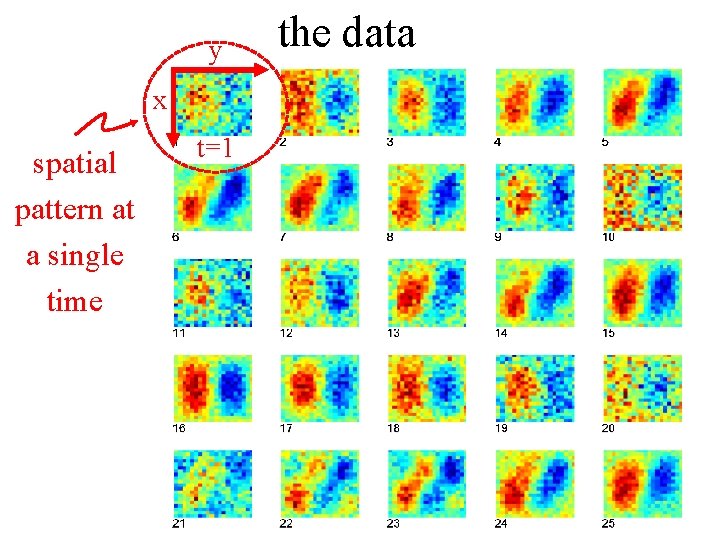
y x spatial pattern at a single time t=1 the data

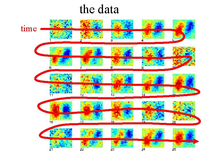
the data time

the data

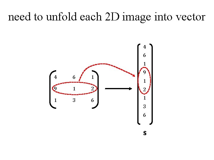
need to unfold each 2 D image into vector 4 6 1 9 1 2 2 1 3 6 1 1 3 6 s

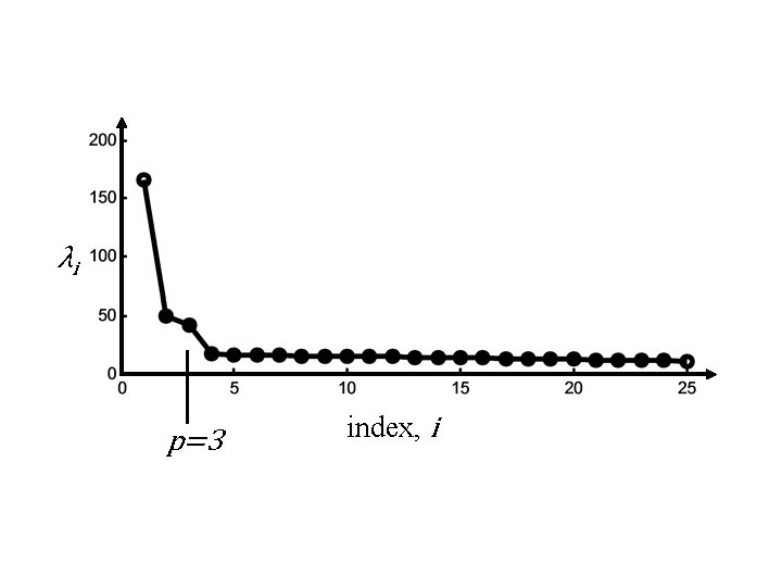
λi p=3 index, i

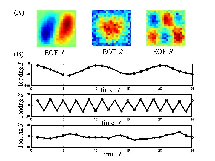
(A) loadng 3 loadng 2 loadng 1 (B) EOF 1 EOF 2 time, t EOF 3

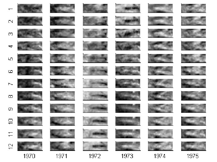
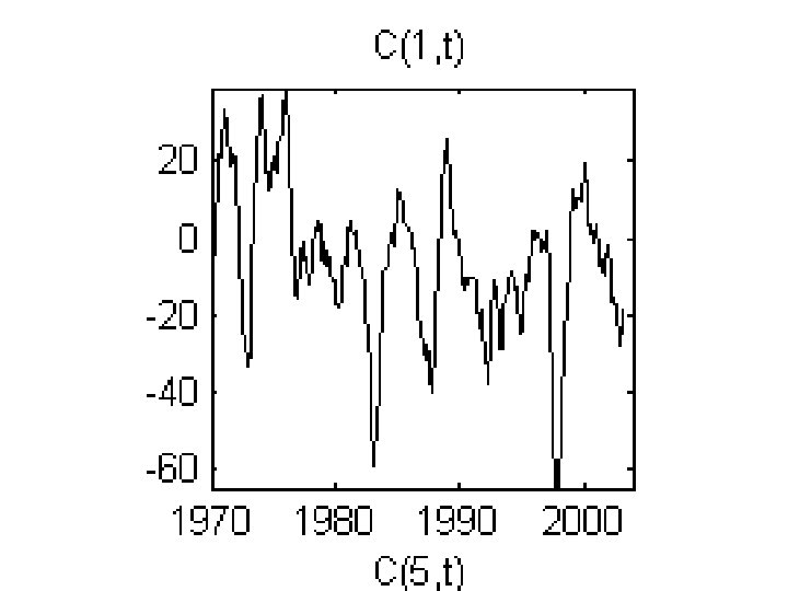
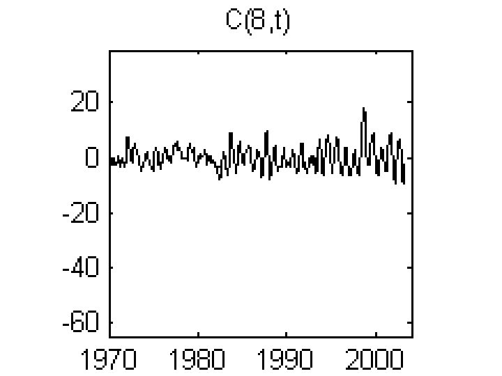
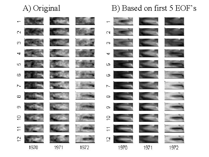
example 3 spatial-temporal patterns (actual data) sea surface temperature in the Pacific Ocean

CAC Sea Surface Temperature 29 N latitude 29 S equatorial Pacific Ocean 124 E longitude 290 E sea surface temperature (black = warm)

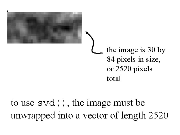
the image is 30 by 84 pixels in size, or 2520 pixels total to use svd(), the image must be unwrapped into a vector of length 2520

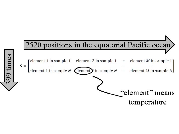
399 times 2520 positions in the equatorial Pacific ocean “element” means temperature

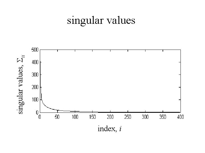
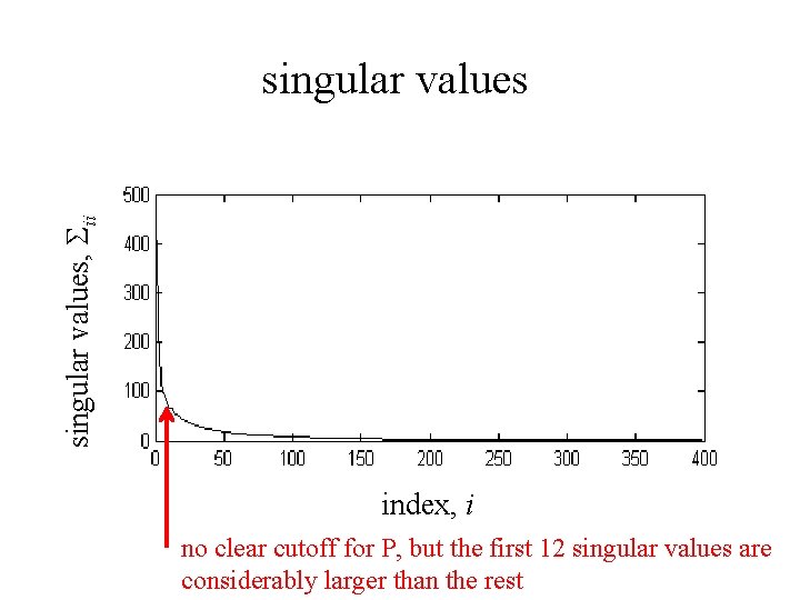
singular values, Sii singular values index, i

singular values, Sii singular values index, i no clear cutoff for P, but the first 12 singular values are considerably larger than the rest

using SVD to approximate data

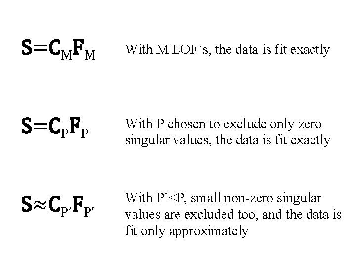
S=CMFM With M EOF’s, the data is fit exactly S=CPFP With P chosen to exclude only zero singular values, the data is fit exactly S≈CP’FP’ With P’<P, small non-zero singular values are excluded too, and the data is fit only approximately

A) Original B) Based on first 5 EOF’s