Lecture 18 Ordinal and Polytomous Logistic Regression BMTRY

Lecture 18 Ordinal and Polytomous Logistic Regression BMTRY 701 Biostatistical Methods II

Categorical Outcomes § Logistic regression is appropriate for binary outcomes § What about other kinds of categorical data? • >2 categories • ordinal data § Standard logistic is not applicable unless you ‘threshold’ the date or collapse categories § BMTRY 711: Analysis of Categorical Data § This is just an overview

Ordinal Logistic Regression § Ordinal Dependent Variable • • • Teaching experience SES (high, middle, low) Degree of Agreement Ability level (e. g. literacy, reading) Severity of disease/outcome Severity of toxicity § Context is important § Example: attitudes towards smoking

Proportional Odds Model § One of several possible regression models for the analysis of ordinal data, and also the most common. § Model predicts the ln(odds) of being in category j or beyond. § Simplifying assumption: “proportional odds” • Effect of covariate assumed to be invariant across splits • Example: 4 categories § 0 vs 1, 2, 3 § 0, 1 vs 2, 3 § 0, 1, 2 vs 3 • Assumes that each of these comparisons yields the same odds ratio

Motivating Example: YTS § The South Carolina Youth Tobacco Survey (SC YTS) is part of the National Youth Tobacco Survey program sponsored by the Centers for Disease Control and Prevention. The YTS is an annual school-based survey designed to evaluate youth-related smoking practices, including initiation and prevalence, cessation, attitudes towards smoking, media influences, and more. The SC YTS is coordinated by the SC Department of Health and Environmental Control and has been administered yearly since 2005. Data for this report are based on years 20052007. The SC YTS uses a two-stage sample cluster design to select a representative sample of public middle (grades 6 -8) and high school (grades 9 -12) students.

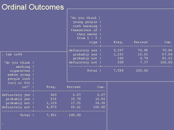
Ordinal Outcomes . tab cr 44 “do you think | young people | risk harming | themselves if | they smoke | from 1 - 5 | ciga | Freq. Percent Cum. --------+-----------------definitely yes | 5, 387 70. 98 probably yes | 1, 283 16. 91 87. 89 probably not | 360 4. 74 92. 63 definitely not | 559 7. 37 100. 00 --------+-----------------Total | 7, 589 100. 00 “do you think | smoking | cigarettes | makes young | people look | cool or fit | in? ” | Freq. Percent Cum. --------+-----------------definitely yes | 460 6. 07 probably yes | 818 10. 79 16. 86 probably not | 1, 329 17. 53 34. 38 definitely not | 4, 975 65. 62 100. 00 --------+-----------------Total | 7, 582 100.

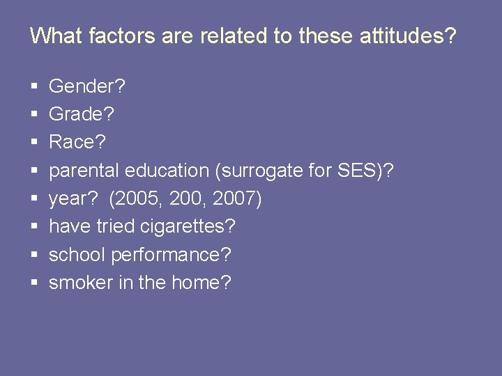
What factors are related to these attitudes? § § § § Gender? Grade? Race? parental education (surrogate for SES)? year? (2005, 2007) have tried cigarettes? school performance? smoker in the home?

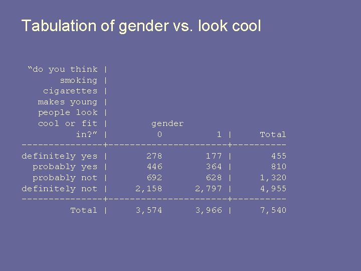
Tabulation of gender vs. look cool “do you think | smoking | cigarettes | makes young | people look | cool or fit | gender in? ” | 0 1 | Total ---------------+---------definitely yes | 278 177 | 455 probably yes | 446 364 | 810 probably not | 692 628 | 1, 320 definitely not | 2, 158 2, 797 | 4, 955 ---------------+---------Total | 3, 574 3, 966 | 7, 540

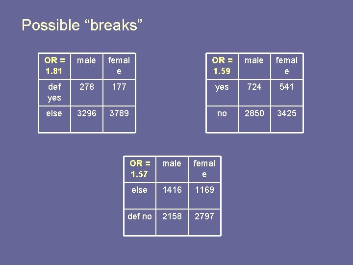
Possible “breaks” OR = 1. 81 male femal e OR = 1. 59 male femal e def yes 278 177 yes 724 541 else 3296 3789 no 2850 3425 OR = 1. 57 male femal e else 1416 1169 def no 2158 2797

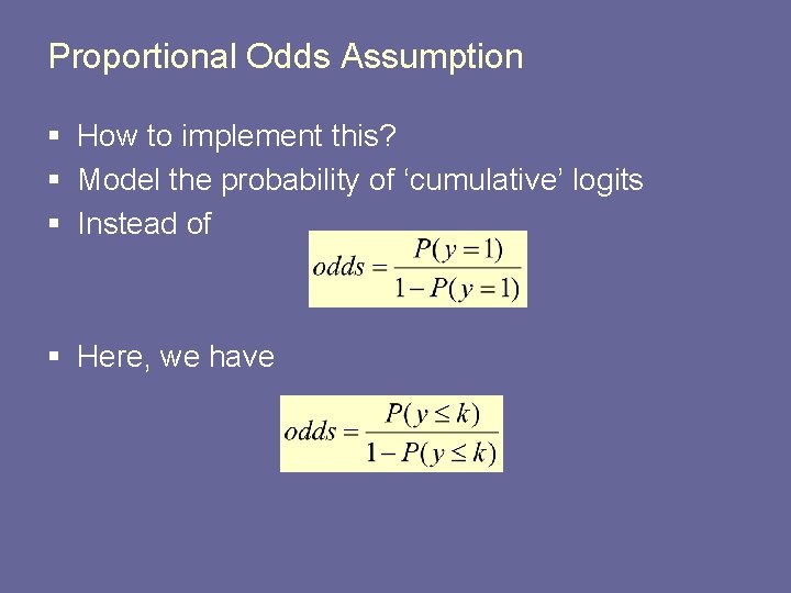
Proportional Odds Assumption § How to implement this? § Model the probability of ‘cumulative’ logits § Instead of § Here, we have

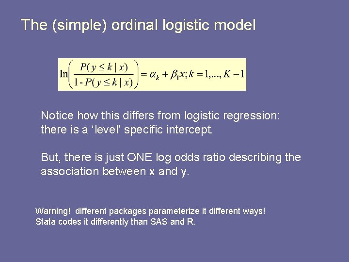
The (simple) ordinal logistic model Notice how this differs from logistic regression: there is a ‘level’ specific intercept. But, there is just ONE log odds ratio describing the association between x and y. Warning! different packages parameterize it different ways! Stata codes it differently than SAS and R.

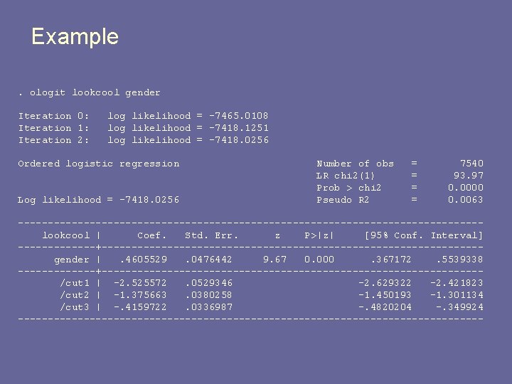
Example. ologit lookcool gender Iteration 0: Iteration 1: Iteration 2: log likelihood = -7465. 0108 log likelihood = -7418. 1251 log likelihood = -7418. 0256 Ordered logistic regression Log likelihood = -7418. 0256 Number of obs LR chi 2(1) Prob > chi 2 Pseudo R 2 = = 7540 93. 97 0. 0000 0. 0063 ---------------------------------------lookcool | Coef. Std. Err. z P>|z| [95% Conf. Interval] -------+--------------------------------gender |. 4605529. 0476442 9. 67 0. 000. 367172. 5539338 -------+--------------------------------/cut 1 | -2. 525572. 0529346 -2. 629322 -2. 421823 /cut 2 | -1. 375663. 0380258 -1. 450193 -1. 301134 /cut 3 | -. 4159722. 0336987 -. 4820204 -. 349924 ---------------------------------------

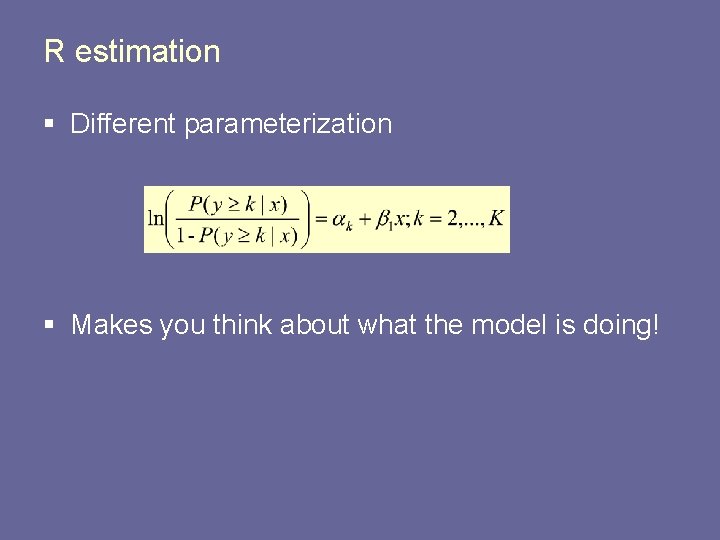
R estimation § Different parameterization § Makes you think about what the model is doing!

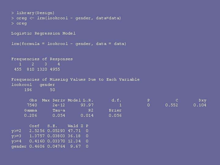
> library(Design) > oreg <- lrm(lookcool ~ gender, data=data) > oreg Logistic Regression Model lrm(formula = lookcool ~ gender, data = data) Frequencies of Responses 1 2 3 4 455 810 1320 4955 Frequencies of Missing Values Due to Each Variable lookcool gender 196 50 Obs 7540 Gamma 0. 206 Max Deriv Model L. R. 2 e-12 93. 97 Tau-a R 2 0. 054 0. 014 Coef y>=2 2. 5256 y>=3 1. 3757 y>=4 0. 4160 gender 0. 4606 S. E. 0. 05293 0. 03803 0. 03370 0. 04764 Wald Z 47. 71 36. 18 12. 34 9. 67 P 0 0 d. f. 1 Brier 0. 056 P 0 C 0. 552 Dxy 0. 104

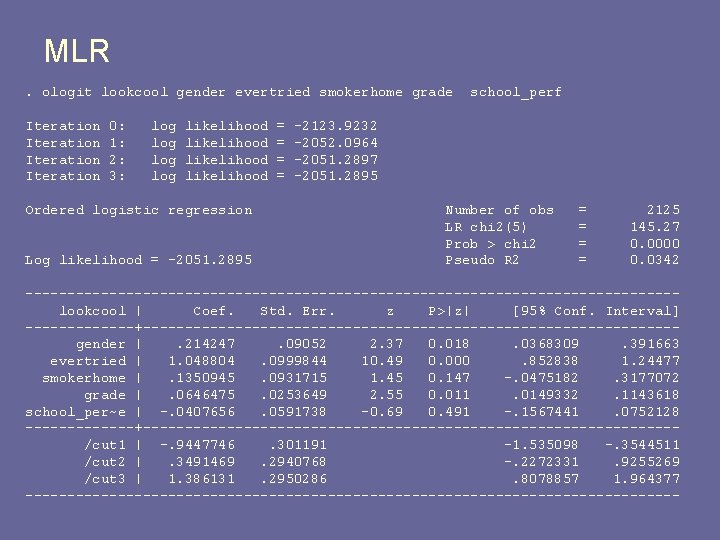
MLR. ologit lookcool gender evertried smokerhome grade Iteration 0: 1: 2: 3: log log likelihood Ordered logistic regression Log likelihood = -2051. 2895 = = school_perf -2123. 9232 -2052. 0964 -2051. 2897 -2051. 2895 Number of obs LR chi 2(5) Prob > chi 2 Pseudo R 2 = = 2125 145. 27 0. 0000 0. 0342 ---------------------------------------lookcool | Coef. Std. Err. z P>|z| [95% Conf. Interval] -------+--------------------------------gender |. 214247. 09052 2. 37 0. 018. 0368309. 391663 evertried | 1. 048804. 0999844 10. 49 0. 000. 852838 1. 24477 smokerhome |. 1350945. 0931715 1. 45 0. 147 -. 0475182. 3177072 grade |. 0646475. 0253649 2. 55 0. 011. 0149332. 1143618 school_per~e | -. 0407656. 0591738 -0. 69 0. 491 -. 1567441. 0752128 -------+--------------------------------/cut 1 | -. 9447746. 301191 -1. 535098 -. 3544511 /cut 2 |. 3491469. 2940768 -. 2272331. 9255269 /cut 3 | 1. 386131. 2950286. 8078857 1. 964377 ---------------------------------------

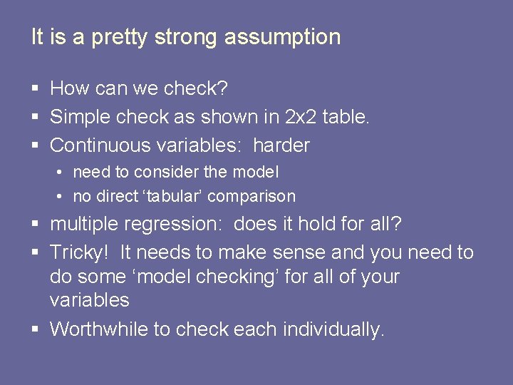
It is a pretty strong assumption § How can we check? § Simple check as shown in 2 x 2 table. § Continuous variables: harder • need to consider the model • no direct ‘tabular’ comparison § multiple regression: does it hold for all? § Tricky! It needs to make sense and you need to do some ‘model checking’ for all of your variables § Worthwhile to check each individually.

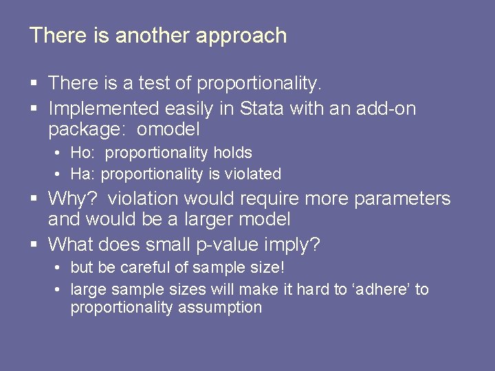
There is another approach § There is a test of proportionality. § Implemented easily in Stata with an add-on package: omodel • Ho: proportionality holds • Ha: proportionality is violated § Why? violation would require more parameters and would be a larger model § What does small p-value imply? • but be careful of sample size! • large sample sizes will make it hard to ‘adhere’ to proportionality assumption

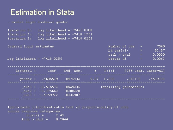
Estimation in Stata. omodel logit lookcool gender Iteration 0: Iteration 1: Iteration 2: log likelihood = -7465. 0108 log likelihood = -7418. 1251 log likelihood = -7418. 0256 Ordered logit estimates Log likelihood = -7418. 0256 Number of obs LR chi 2(1) Prob > chi 2 Pseudo R 2 = = 7540 93. 97 0. 0000 0. 0063 ---------------------------------------lookcool | Coef. Std. Err. z P>|z| [95% Conf. Interval] -------+--------------------------------gender |. 4605529. 0476442 9. 67 0. 000. 367172. 5539338 -------+--------------------------------_cut 1 | -2. 525572. 0529346 (Ancillary parameters) _cut 2 | -1. 375663. 0380258 _cut 3 | -. 4159722. 0336987 ---------------------------------------Approximate likelihood-ratio test of proportionality of odds across response categories: chi 2(2) = 2. 43 Prob > chi 2 = 0. 2964

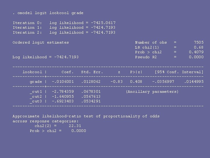
. omodel logit lookcool grade Iteration 0: Iteration 1: Iteration 2: log likelihood = -7425. 0617 log likelihood = -7424. 7193 Ordered logit estimates Log likelihood = -7424. 7193 Number of obs LR chi 2(1) Prob > chi 2 Pseudo R 2 = = 7505 0. 68 0. 4079 0. 0000 ---------------------------------------lookcool | Coef. Std. Err. z P>|z| [95% Conf. Interval] -------+--------------------------------grade | -. 0106001. 0128062 -0. 83 0. 408 -. 0356997. 0144995 -------+--------------------------------_cut 1 | -2. 784359. 0678301 (Ancillary parameters) _cut 2 | -1. 640955. 0567613 _cut 3 | -. 6923403. 0534291 ---------------------------------------Approximate likelihood-ratio test of proportionality of odds across response categories: chi 2(2) = 22. 31 Prob > chi 2 = 0. 0000

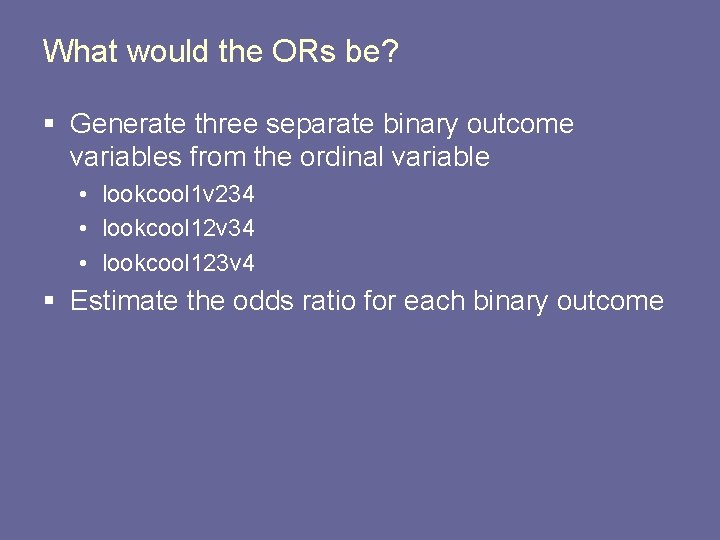
What would the ORs be? § Generate three separate binary outcome variables from the ordinal variable • lookcool 1 v 234 • lookcool 12 v 34 • lookcool 123 v 4 § Estimate the odds ratio for each binary outcome

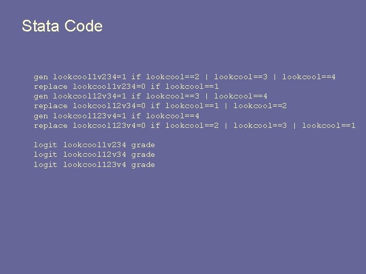
Stata Code gen lookcool 1 v 234=1 if lookcool==2 | lookcool==3 | lookcool==4 replace lookcool 1 v 234=0 if lookcool==1 gen lookcool 12 v 34=1 if lookcool==3 | lookcool==4 replace lookcool 12 v 34=0 if lookcool==1 | lookcool==2 gen lookcool 123 v 4=1 if lookcool==4 replace lookcool 123 v 4=0 if lookcool==2 | lookcool==3 | lookcool==1 logit lookcool 1 v 234 grade logit lookcool 12 v 34 grade logit lookcool 123 v 4 grade

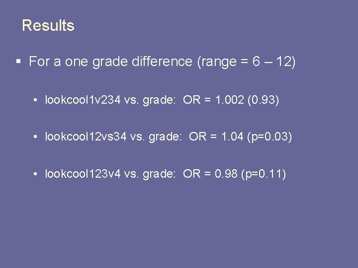
Results § For a one grade difference (range = 6 – 12) • lookcool 1 v 234 vs. grade: OR = 1. 002 (0. 93) • lookcool 12 vs 34 vs. grade: OR = 1. 04 (p=0. 03) • lookcool 123 v 4 vs. grade: OR = 0. 98 (p=0. 11)

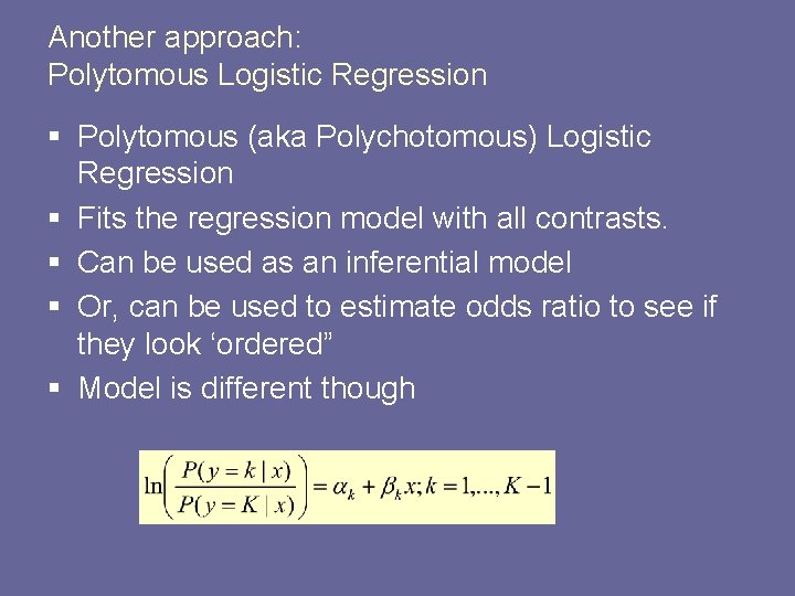
Another approach: Polytomous Logistic Regression § Polytomous (aka Polychotomous) Logistic Regression § Fits the regression model with all contrasts. § Can be used as an inferential model § Or, can be used to estimate odds ratio to see if they look ‘ordered” § Model is different though

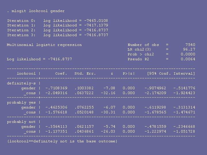
. mlogit lookcool gender Iteration 0: 1: 2: 3: log log likelihood = = Multinomial logistic regression Log likelihood = -7416. 8737 -7465. 0108 -7417. 1379 -7416. 8737 Number of obs LR chi 2(3) Prob > chi 2 Pseudo R 2 = = 7540 96. 27 0. 0000 0. 0064 ---------------------------------------lookcool | Coef. Std. Err. z P>|z| [95% Conf. Interval] -------+--------------------------------definitely~s | gender | -. 7108369. 1003382 -7. 08 0. 000 -. 9074962 -. 5141776 _cons | -2. 049316. 0637222 -32. 16 0. 000 -2. 174209 -1. 924423 -------+--------------------------------probably yes | gender | -. 4625306. 0762255 -6. 07 0. 000 -. 6119298 -. 3131314 _cons | -1. 576618. 0520148 -30. 31 0. 000 -1. 678565 -1. 474671 -------+--------------------------------probably not | gender | -. 3564113. 0621157 -5. 74 0. 000 -. 4781559 -. 2346668 _cons | -1. 137351. 0436861 -26. 03 0. 000 -1. 222974 -1. 051728 ---------------------------------------(lookcool==definitely not is the base outcome)

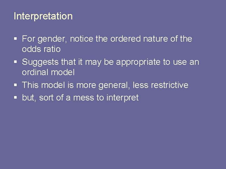
Interpretation § For gender, notice the ordered nature of the odds ratio § Suggests that it may be appropriate to use an ordinal model § This model is more general, less restrictive § but, sort of a mess to interpret

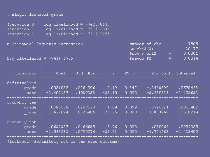
. mlogit lookcool grade Iteration 0: Iteration 1: Iteration 2: log likelihood = -7425. 0617 log likelihood = -7414. 6932 log likelihood = -7414. 6755 Multinomial logistic regression Log likelihood = -7414. 6755 Number of obs LR chi 2(3) Prob > chi 2 Pseudo R 2 = = 7505 20. 77 0. 0001 0. 0014 ---------------------------------------lookcool | Coef. Std. Err. z P>|z| [95% Conf. Interval] -------+--------------------------------definitely~s | grade |. 0051085. 0264996 0. 19 0. 847 -. 0468299. 0570468 _cons | -2. 407127. 1089328 -22. 10 0. 000 -2. 620632 -2. 193623 -------+--------------------------------probably yes | grade | -. 0390659. 0207178 -1. 89 0. 059 -. 0796721. 0015402 _cons | -1. 672094. 0825905 -20. 25 0. 000 -1. 833968 -1. 510219 -------+--------------------------------probably not | grade |. 0627357. 0166685 3. 76 0. 000. 030066. 0954055 _cons | -1. 562533. 0709374 -22. 03 0. 000 -1. 701568 -1. 423499 ---------------------------------------(lookcool==definitely not is the base outcome)

In R? § mlogit library § requires a data transformation step