Lecture 17 String Matching Cp Sc 212 Algorithms

Lecture 17. String Matching Cp. Sc 212: Algorithms and Data Structures Brian C. Dean School of Computing Clemson University Fall, 2012

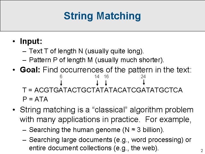
String Matching • Input: – Text T of length N (usually quite long). – Pattern P of length M (usually much shorter). • Goal: Find occurrences of the pattern in the text: 6 14 16 24 T = ACGTGATACTGCTATATACATCGATATGCTCA P = ATA • String matching is a “classical” algorithm problem with many applications in practice. For example, – Searching the human genome (N ≈ 3 billion). – Searching large documents (e. g. , word processing) or entire document collections (e. g. , the web). 2

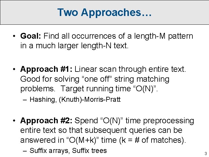
Two Approaches… • Goal: Find all occurrences of a length-M pattern in a much larger length-N text. • Approach #1: Linear scan through entire text. Good for solving “one off” string matching problems. Target running time “O(N)”. – Hashing, (Knuth)-Morris-Pratt • Approach #2: Spend “O(N)” time preprocessing entire text so that subsequent queries can be answered in “O(M+k)” time (k = # of matches). – Suffix arrays, Suffix trees 3

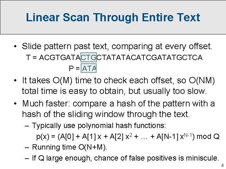
Linear Scan Through Entire Text • Slide pattern past text, comparing at every offset. T = ACGTGATACTGCTATATACATCGATATGCTCA P = ATA • It takes O(M) time to check each offset, so O(NM) total time is easy to obtain, but usually too slow. • Much faster: compare a hash of the pattern with a hash of the sliding window through the text. – Typically use polynomial hash functions: p(x) = (A[0] + A[1] x + A[2] x 2 + … + A[N-1] x. N-1) mod Q – Running time O(N+M). – If Q large enough, chance of false positives is miniscule. 4

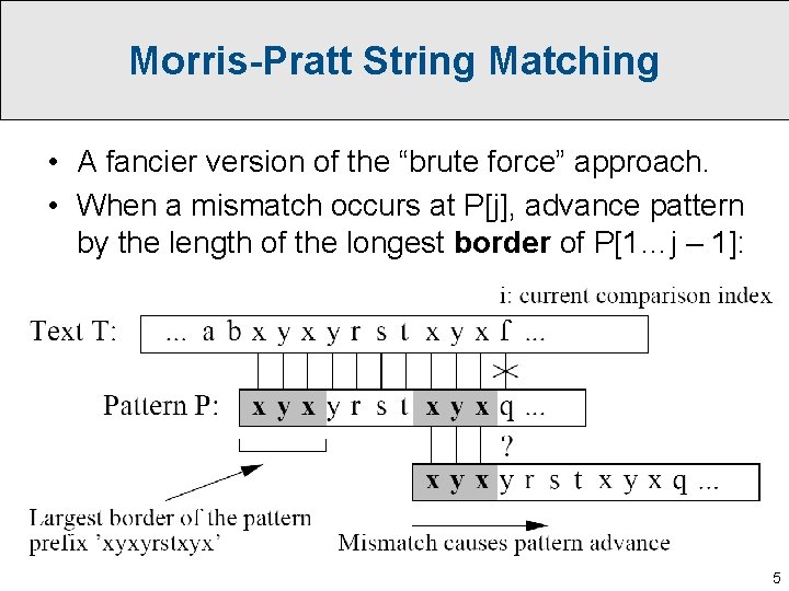
Morris-Pratt String Matching • A fancier version of the “brute force” approach. • When a mismatch occurs at P[j], advance pattern by the length of the longest border of P[1…j – 1]: 5

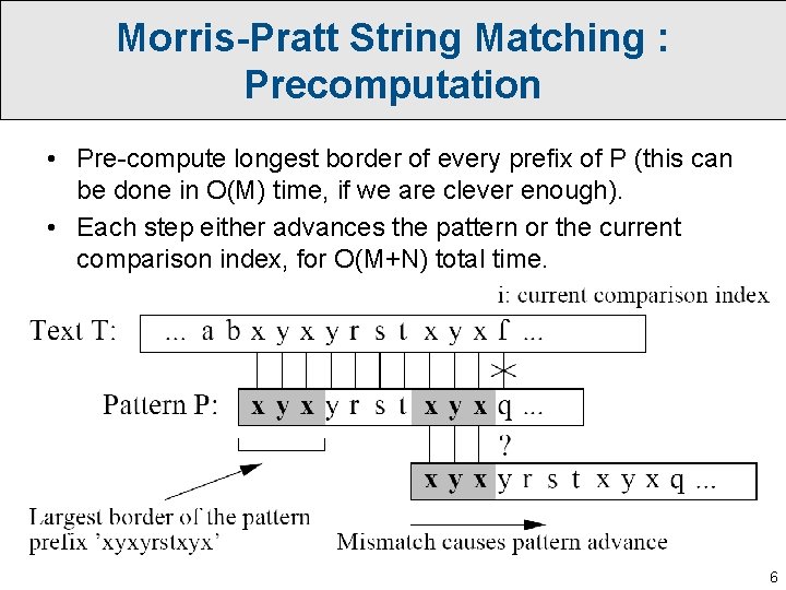
Morris-Pratt String Matching : Precomputation • Pre-compute longest border of every prefix of P (this can be done in O(M) time, if we are clever enough). • Each step either advances the pattern or the current comparison index, for O(M+N) total time. 6

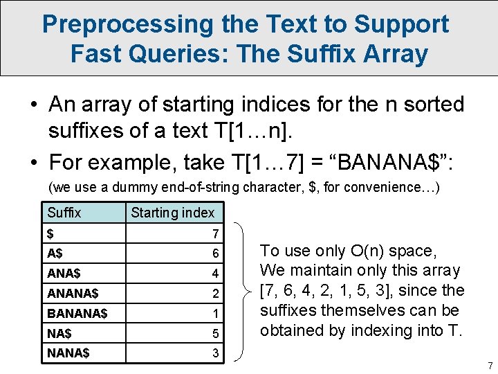
Preprocessing the Text to Support Fast Queries: The Suffix Array • An array of starting indices for the n sorted suffixes of a text T[1…n]. • For example, take T[1… 7] = “BANANA$”: (we use a dummy end-of-string character, $, for convenience…) Suffix Starting index $ 7 A$ 6 ANA$ 4 ANANA$ 2 BANANA$ 1 NA$ 5 NANA$ 3 To use only O(n) space, We maintain only this array [7, 6, 4, 2, 1, 5, 3], since the suffixes themselves can be obtained by indexing into T. 7

Searching a Suffix Array • A pattern P[1…M] will match a contiguous range of entries in the suffix array. • Use binary search in O(M log N) time to locate the endpoints Suffix Starting index of this range. $ 7 • Then O(1) time per A$ 6 index to enumerate ANA$ 4 all matches. ANANA$ 2 1 • Example: the pattern BANANA$ 5 P = “ANA” matches NANA$ 3 at indices 2 and 4. 8

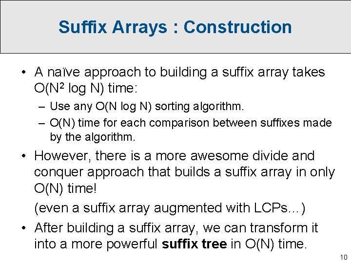
Suffix Arrays : Construction • A naïve approach to building a suffix array takes O(N 2 log N) time: – Use any O(N log N) sorting algorithm. – O(N) time for each comparison between suffixes made by the algorithm. • However, there is a more awesome divide and conquer approach that builds a suffix array in only O(N) time! (even a suffix array augmented with LCPs…) • After building a suffix array, we can transform it into a more powerful suffix tree in O(N) time. 10

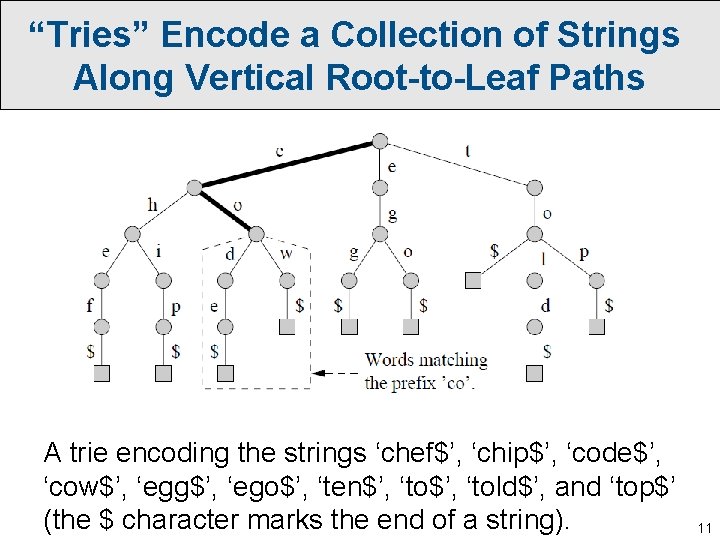
“Tries” Encode a Collection of Strings Along Vertical Root-to-Leaf Paths A trie encoding the strings ‘chef$’, ‘chip$’, ‘code$’, ‘cow$’, ‘egg$’, ‘ego$’, ‘ten$’, ‘told$’, and ‘top$’ (the $ character marks the end of a string). 11

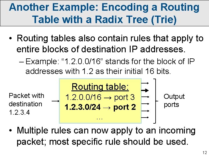
Another Example: Encoding a Routing Table with a Radix Tree (Trie) • Routing tables also contain rules that apply to entire blocks of destination IP addresses. – Example: “ 1. 2. 0. 0/16” stands for the block of IP addresses with 1. 2 as their initial 16 bits. Packet with destination 1. 2. 3. 4 Routing table: 1. 2. 0. 0/16 → port 3 1. 2. 3. 0/24 → port 2 … Output ports • Multiple rules can now apply to an incoming packet; most specific rule should be used. 12

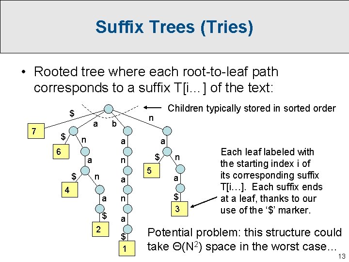
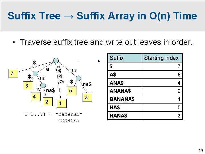
Suffix Trees (Tries) • Rooted tree where each root-to-leaf path corresponds to a suffix T[i…] of the text: $ 7 a $ 6 a a $ n b n Children typically stored in sorted order a $ n n 4 2 a a n $ a $ 1 5 n a $ 3 Each leaf labeled with the starting index i of its corresponding suffix T[i…]. Each suffix ends at a leaf, thanks to our use of the ‘$’ marker. Potential problem: this structure could take Θ(N 2) space in the worst case… 13

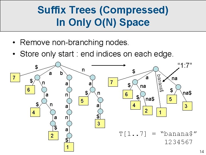
Suffix Trees (Compressed) In Only O(N) Space • Remove non-branching nodes. • Store only start : end indices on each edge. $ $ b n 6 $ $ a a n 4 2 a a n $ a $ 1 7 a $ n 5 “ 1: 7” n a $ 3 a $ na 6 $ 4 $ banana 7 a n na$ 2 na $ na$ 5 3 1 T[1. . 7] = “banana$” 1234567 14

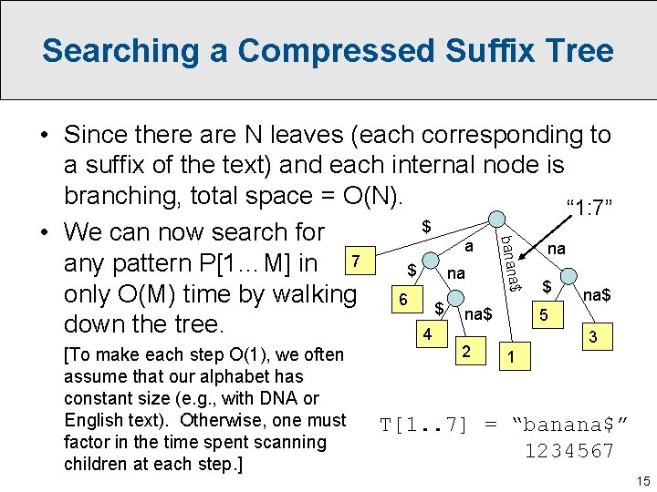
Searching a Compressed Suffix Tree $ banana • Since there are N leaves (each corresponding to a suffix of the text) and each internal node is branching, total space = O(N). “ 1: 7” $ • We can now search for a na any pattern P[1…M] in 7 $ na$ only O(M) time by walking 6 $ na$ 5 down the tree. 4 3 [To make each step O(1), we often assume that our alphabet has constant size (e. g. , with DNA or English text). Otherwise, one must factor in the time spent scanning children at each step. ] 2 1 T[1. . 7] = “banana$” 1234567 15

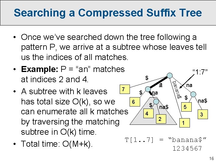
Searching a Compressed Suffix Tree na$ a ban • Once we’ve searched down the tree following a pattern P, we arrive at a subtree whose leaves tell us the indices of all matches. • Example: P = “an” matches “ 1: 7” $ at indices 2 and 4. a na 7 • A subtree with k leaves $ na$ 6 has total size O(k), so we $ na$ 5 can enumerate all k matches 4 3 2 by traversing the matching 1 subtree in O(k) time. T[1. . 7] = “banana$” • Total time: O(M+k). 1234567 16

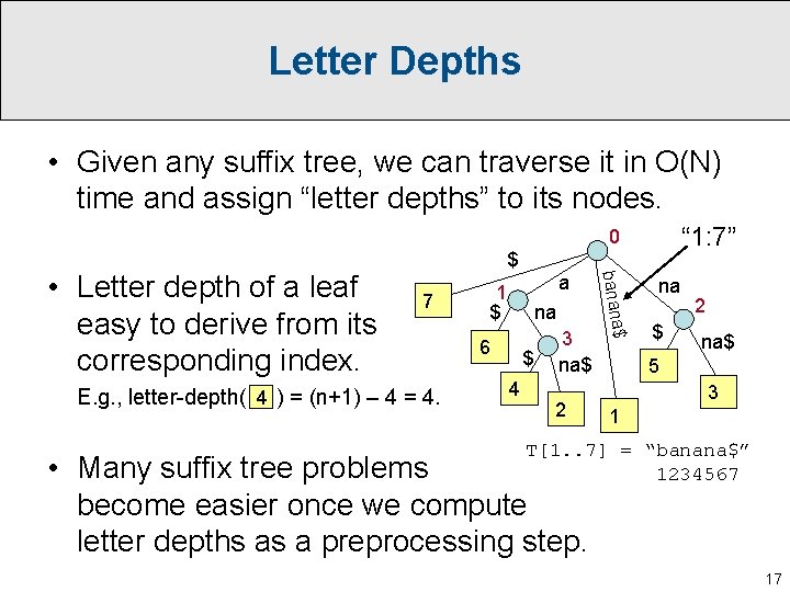
Letter Depths • Given any suffix tree, we can traverse it in O(N) time and assign “letter depths” to its nodes. “ 1: 7” 0 7 E. g. , letter-depth( 4 ) = (n+1) – 4 = 4. a 1 $ na 6 $ 4 3 na$ 2 $ banana • Letter depth of a leaf easy to derive from its corresponding index. $ na $ 2 na$ 5 3 1 T[1. . 7] = “banana$” 1234567 • Many suffix tree problems become easier once we compute letter depths as a preprocessing step. 17

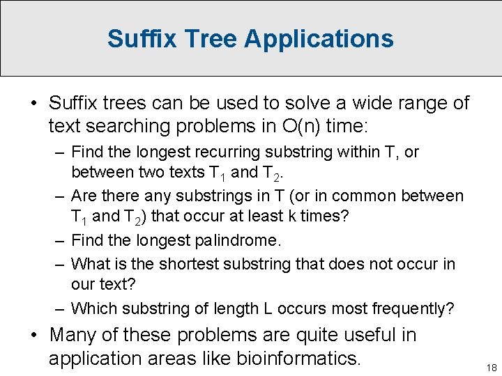
Suffix Tree Applications • Suffix trees can be used to solve a wide range of text searching problems in O(n) time: – Find the longest recurring substring within T, or between two texts T 1 and T 2. – Are there any substrings in T (or in common between T 1 and T 2) that occur at least k times? – Find the longest palindrome. – What is the shortest substring that does not occur in our text? – Which substring of length L occurs most frequently? • Many of these problems are quite useful in application areas like bioinformatics. 18

Suffix Tree → Suffix Array in O(n) Time • Traverse suffix tree and write out leaves in order. Suffix $ $ na $ banana 7 a 6 $ 4 na$ 2 na $ na$ 5 3 1 T[1. . 7] = “banana$” 1234567 Starting index $ 7 A$ 6 ANA$ 4 ANANA$ 2 BANANA$ 1 NA$ 5 NANA$ 3 19

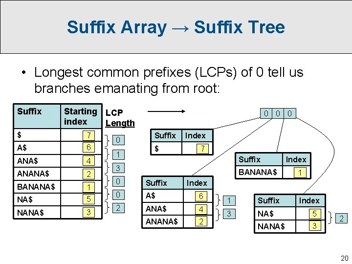
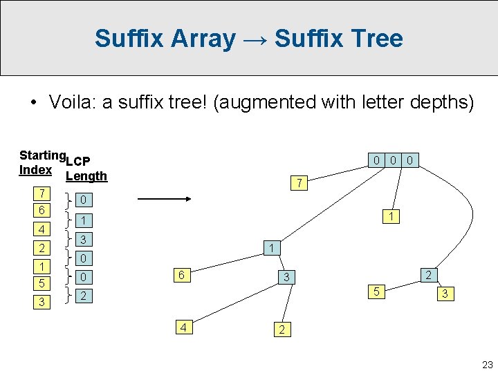
Suffix Array → Suffix Tree • Longest common prefixes (LCPs) of 0 tell us branches emanating from root: Suffix Starting LCP index Length $ 7 A$ 6 ANA$ 4 ANANA$ 2 BANANA$ 1 NA$ 5 NANA$ 3 0 1 0 0 0 Suffix $ Index 7 Suffix 3 BANANA$ 0 Suffix 0 A$ 6 2 ANA$ 4 ANANA$ 2 Index 1 Suffix 3 NA$ 5 NANA$ 3 Index 2 20

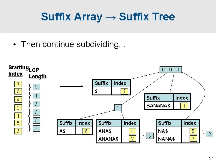
Suffix Array → Suffix Tree • Then continue subdividing… Starting LCP Index Length 7 6 4 2 1 5 3 0 0 0 Suffix 0 $ 1 7 Suffix 3 2 BANANA$ 1 0 0 Index Suffix A$ ANA$ 4 ANANA$ 2 6 Index Suffix 3 Index 1 Index NA$ 5 NANA$ 3 2 21

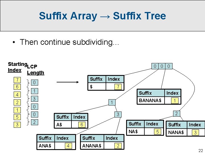
Suffix Array → Suffix Tree • Then continue subdividing… Starting LCP Index Length 7 6 4 2 1 5 3 0 0 0 Suffix 0 Index $ 1 7 Suffix 3 BANANA$ 1 0 0 Suffix Index 2 A$ Suffix NA$ Index ANA$ 4 Suffix ANANA$ 1 2 3 6 Suffix Index 5 Suffix NANA$ Index 3 Index 2 22

Suffix Array → Suffix Tree • Voila: a suffix tree! (augmented with letter depths) Starting LCP Index Length 7 6 4 2 1 5 3 0 0 0 7 0 1 1 3 1 0 0 6 2 3 5 2 4 3 2 23

Your Next Assignment… • Process 25 MB of text (pulled from social media postings related to technology and algorithms over the course of a month) to do predictive text completion. • How can we do this effectively using suffix trees? 24