Lecture 17 Portfolio Selection John Rundle Econophysics PHYS

Lecture 17 Portfolio Selection John Rundle Econophysics PHYS 250

Efficient Market Hypothesis https: //en. wikipedia. org/wiki/Efficient-market_hypothesis • • • In financial economics, the efficient-market hypothesis (EMH) states that asset prices fully reflect all available information. A direct implication is that it is impossible to "beat the market" consistently on a risk-adjusted basis since market prices should only react to new information or changes in discount rates (the latter may be predictable or unpredictable). The EMH was developed by Professor Eugene Fama who argued that stocks always trade at their fair value, making it impossible for investors to either purchase undervalued stocks or sell stocks for inflated prices. In physics, this would be the “assume a spherical cow” idea Under the EMH, it should be impossible to outperform the overall market through expert stock selection or market timing, and that the only way an investor can possibly obtain higher returns is by chance or by purchasing riskier investments His 2012 study with Kenneth French confirmed this view, showing that the distribution of abnormal returns of US mutual funds is very similar to what would be expected if no fund managers had any skill—a necessary condition for the EMH to hold.

Efficient Market Hypothesis https: //en. wikipedia. org/wiki/Efficient-market_hypothesis • • • There are three variants of the hypothesis: "weak, " "semi-strong, " and "strong" form. The weak form of the EMH claims that prices on traded assets (e. g. , stocks, bonds, or property) already reflect all past publicly available information. The semi-strong form of the EMH claims both that prices reflect all publicly available information and that prices instantly change to reflect new public information. The strong form of the EMH additionally claims that prices instantly reflect even hidden "insider" information. Critics have blamed the belief in rational markets for much of the 2008 -2009 financial crisis. In response, proponents of the hypothesis have stated that market efficiency does not mean not having any uncertainty about the future, that market efficiency is a simplification of the world which may not always hold true, and that the market is practically efficient for investment purposes for most individuals.

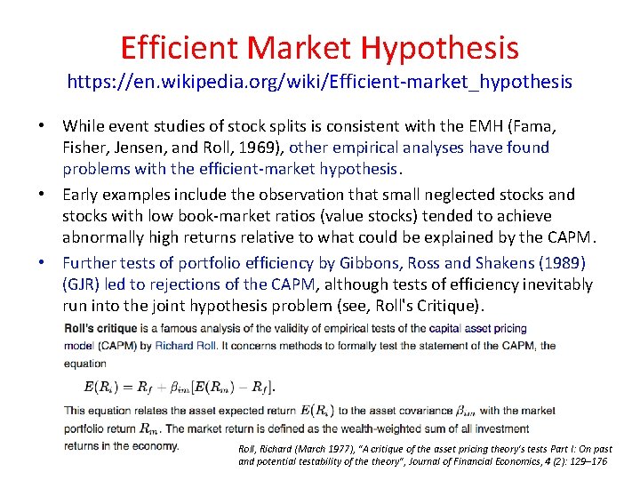
Efficient Market Hypothesis https: //en. wikipedia. org/wiki/Efficient-market_hypothesis • While event studies of stock splits is consistent with the EMH (Fama, Fisher, Jensen, and Roll, 1969), other empirical analyses have found problems with the efficient-market hypothesis. • Early examples include the observation that small neglected stocks and stocks with low book-market ratios (value stocks) tended to achieve abnormally high returns relative to what could be explained by the CAPM. • Further tests of portfolio efficiency by Gibbons, Ross and Shakens (1989) (GJR) led to rejections of the CAPM, although tests of efficiency inevitably run into the joint hypothesis problem (see, Roll's Critique). Roll, Richard (March 1977), "A critique of the asset pricing theory's tests Part I: On past and potential testability of theory", Journal of Financial Economics, 4 (2): 129– 176

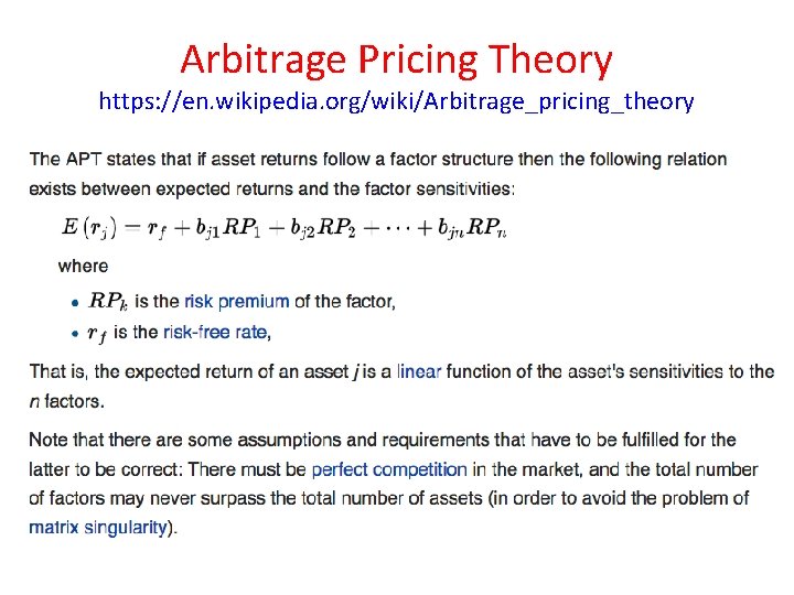
Arbitrage Pricing Theory https: //en. wikipedia. org/wiki/Arbitrage_pricing_theory • In finance, arbitrage pricing theory (APT) is a general theory of asset pricing that holds that the expected return of a financial asset can be modeled as a linear function of various macro-economic factors or theoretical market indices • Sensitivity to changes in each factor is represented by a factor-specific beta coefficient. • The model-derived rate of return will then be used to price the asset correctly—the asset price should equal the expected end of period price discounted at the rate implied by the model. • If the price diverges, arbitrage should bring it back into line. • The theory was proposed by the economist Stephen Ross in 1976.

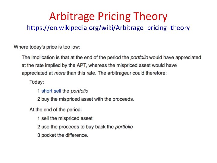
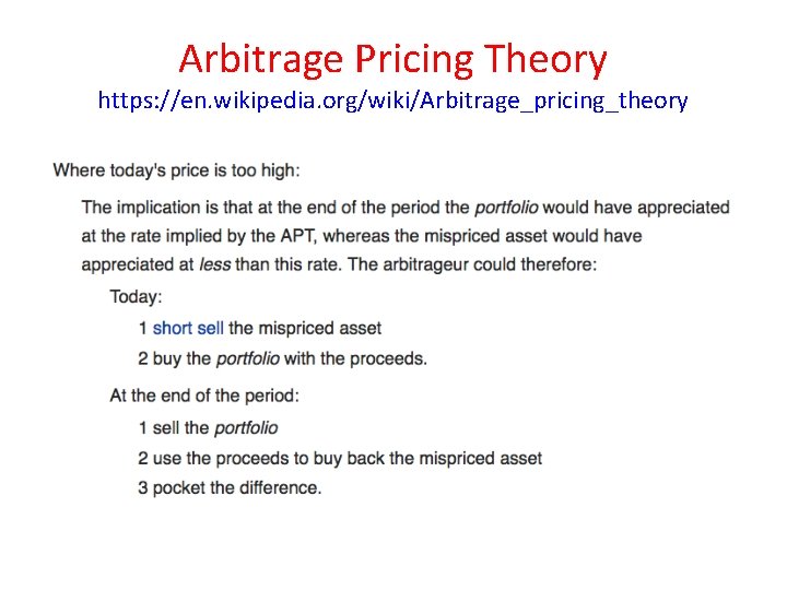
Arbitrage Pricing Theory https: //en. wikipedia. org/wiki/Arbitrage_pricing_theory • Arbitrage consists of trading in two assets – with at least one being mispriced. • I. e. , there is an assumption that we have a “correctly priced” portfolio from a factor model, and a mispriced asset • The arbitrageur sells the asset which is relatively too expensive and uses the proceeds to buy one which is relatively too cheap. • Under the APT, an asset is mispriced if its current price diverges from the price predicted by the model. • The asset price today should equal the sum of all future cash flows discounted at the APT rate, where the expected return of the asset is a linear function of various factors, and sensitivity to changes in each factor is represented by a factor-specific beta coefficient.

Arbitrage Pricing Theory https: //en. wikipedia. org/wiki/Arbitrage_pricing_theory • A correctly priced asset here may be in fact a synthetic asset - a portfolio consisting of other correctly priced assets. • This portfolio has the same exposure to each of the macroeconomic factors as the mispriced asset. • The arbitrageur creates the portfolio by identifying X correctly priced assets (one per factor plus one) and then weighting the assets such that portfolio beta per factor is the same as for the mispriced asset. • When the investor is long the asset and short the portfolio (or vice versa) she has created a position which has a positive expected return (the difference between asset return and portfolio return) • She also has a net-zero exposure to any macroeconomic factor and the position is therefore risk free (other than for firm specific risk). • The arbitrageur is thus in a position to make a risk-free profit

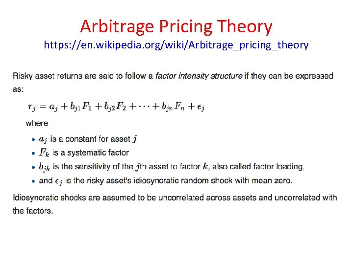
Arbitrage Pricing Theory https: //en. wikipedia. org/wiki/Arbitrage_pricing_theory

Arbitrage Pricing Theory https: //en. wikipedia. org/wiki/Arbitrage_pricing_theory

Arbitrage Pricing Theory https: //en. wikipedia. org/wiki/Arbitrage_pricing_theory

Arbitrage Pricing Theory https: //en. wikipedia. org/wiki/Arbitrage_pricing_theory

Arbitrage Pricing Theory https: //en. wikipedia. org/wiki/Arbitrage_pricing_theory • The APT along with the capital asset pricing model (CAPM) is one of two influential theories on asset pricing. • The APT differs from the CAPM in that it is less restrictive in its assumptions. • It allows for an explanatory (as opposed to statistical) model of asset returns. • It assumes that each investor will hold a unique portfolio with its own particular array of betas, as opposed to the identical "market portfolio". In some ways, the CAPM can be considered a "special case" of the APT in that the securities market line represents a single-factor model of the asset price, where beta is exposed to changes in value of the market.

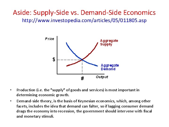
Aside: Supply-Side vs. Demand-Side Economics http: //www. investopedia. com/articles/05/011805. asp • • Production (i. e. the "supply" of goods and services) is most important in determining economic growth. Demand-side theory, is the basis of Keynesian economics, which, among other facets, includes the idea that demand can falter, so if lagging consumer demand drags the economy into recession, the government should intervene with fiscal and monetary stimuli.

Arbitrage Pricing Theory https: //en. wikipedia. org/wiki/Arbitrage_pricing_theory • Additionally, the APT can be seen as a "supply-side" model, since its beta coefficients reflect the sensitivity of the underlying asset to economic factors. • Thus, factor shocks would cause structural changes in assets' expected returns, or in the case of stocks, in firms' profits (firms are considered to be the “suppliers” of the assets). • On the other side, the capital asset pricing model is considered a "demand side" model. • Its results, although similar to those of the APT, arise from a maximization problem of each investor's utility function, and from the resulting market equilibrium (investors are considered to be the "consumers" of the assets).

Arbitrage Pricing Theory: Factors https: //en. wikipedia. org/wiki/Arbitrage_pricing_theory • • • As with the CAPM, the factor-specific betas are found via a linear regression of historical security returns on the factor in question. Unlike the CAPM, in the APT, the number and nature of these factors is likely to change over time and between economies. As a result, this issue is essentially empirical in nature. Several a priori guidelines as to the characteristics required of potential factors are, however, suggested: • They should represent undiversifiable influences (these are, clearly, more likely to be macroeconomic rather than firm-specific in nature) • Timely and accurate information on these variables is required • The relationship should be theoretically justifiable on economic grounds

Arbitrage Pricing Theory: Factors https: //en. wikipedia. org/wiki/Arbitrage_pricing_theory Chen, Roll and Ross (1986) identified the following macroeconomic factors as significant in explaining security returns: – Surprises in inflation; – Surprises in GDP as indicated by an industrial production index; – Surprises in investor confidence due to changes in default premium in corporate bonds; – Surprise shifts in the yield curve. – FED announcements

Arbitrage Pricing Theory: Factors https: //en. wikipedia. org/wiki/Arbitrage_pricing_theory As a practical matter, indices or spot or futures market prices may be used in place of macro-economic factors, which are reported at low frequency (e. g. monthly) and often with significant estimation errors. • Market indices are sometimes derived by means of factor analysis. • More direct "indices" that might be used are: 1. 2. 3. 4. 5. 6. Short-term interest rates; The difference in long-term and short-term interest rates; A diversified stock index such as the S&P 500 or NYSE Composite; Oil prices Gold or other precious metal prices Currency exchange rates

Factor Analysis and PCA https: //en. wikipedia. org/wiki/Factor_analysis • Factor analysis is related to principal component analysis (PCA), but the two are not identical. • There has been significant controversy in the field over differences between the two techniques (see section on exploratory factor analysis versus principal components analysis). • PCA is a more basic version of exploratory factor analysis (EFA) that was developed in the early days prior to the advent of high-speed computers.

Aside: Principal Component Analysis https: //en. wikipedia. org/wiki/Principal_component_analysis • Principal Component Analysis (PCA) is a statistical procedure that uses an orthogonal transformation to convert a set of observations of possibly correlated variables into a set of values of linearly uncorrelated variables called principal components. • The number of principal components is less than or equal to the number of original variables. • This transformation is defined in such a way that the first principal component has the largest possible variance (that is, accounts for as much of the variability in the data as possible) • Each succeeding component in turn has the highest variance possible under the constraint that it is orthogonal to the preceding components. • The resulting vectors are an uncorrelated orthogonal basis set. • PCA is sensitive to the relative scaling of the original variables.

Aside: Principal Component Analysis https: //en. wikipedia. org/wiki/Principal_component_analysis • • • PCA is mostly used as a tool in exploratory data analysis and for making predictive models. PCA can be done by eigenvalue decomposition of a data covariance (or correlation) matrix or singular value decomposition of a data matrix, usually after mean centering (and normalizing or using Z-scores) the data matrix for each attribute. The results of a PCA are usually discussed in terms of component scores, sometimes called factor scores (the transformed variable values corresponding to a particular data point), and loadings (the weight by which each standardized original variable should be multiplied to get the component score).

Factor Analysis: Methods https: //en. wikipedia. org/wiki/Factor_analysis • Factor analysis is a statistical method used to describe variability among observed, correlated variables in terms of a potentially lower number of unobserved variables called factors. • For example, it is possible that variations in six observed variables mainly reflect the variations in two unobserved (underlying) variables. • Factor analysis searches for such joint variations in response to unobserved latent variables. • The observed variables are modeled as linear combinations of the potential factors, plus "error" terms. • Factor analysis aims to find independent latent variables.

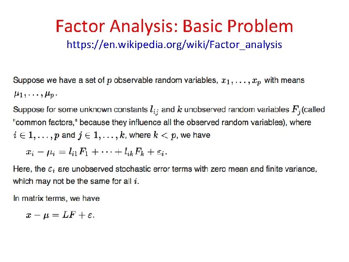
Factor Analysis: Basic Problem https: //en. wikipedia. org/wiki/Factor_analysis

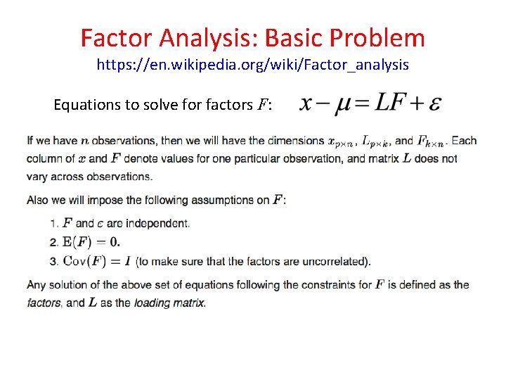
Factor Analysis: Basic Problem https: //en. wikipedia. org/wiki/Factor_analysis Equations to solve for factors F:

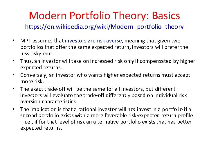
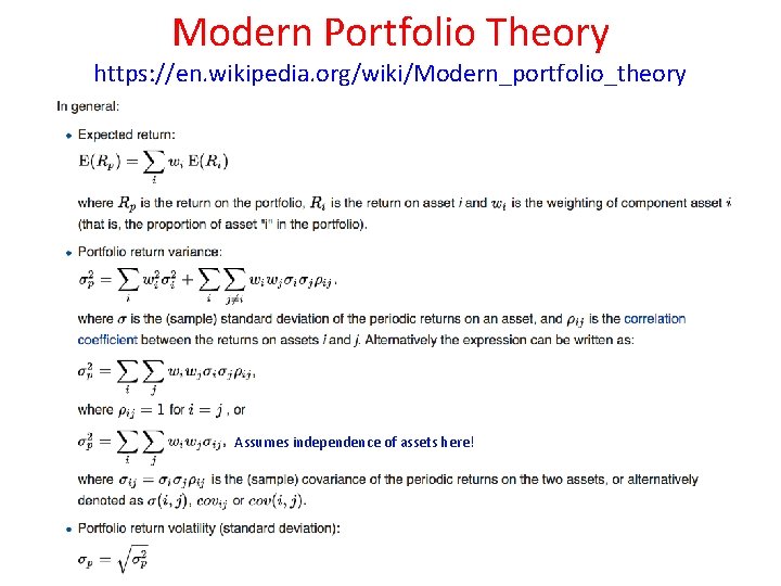
Modern Portfolio Theory: Basics https: //en. wikipedia. org/wiki/Modern_portfolio_theory Modern Portfolio Theory (MPT), or mean-variance analysis, is a mathematical framework for assembling a portfolio of assets such that the expected return is maximized for a given level of risk, defined as variance. • Its key insight is that an asset's risk and return should not be assessed by itself, but by how it contributes to a portfolio's overall risk and return. • Economist Harry Markowitz introduced MPT in a 1952 essay, for which he was later awarded a Nobel Prize in economics. Under the model: 1. Portfolio return is the proportion-weighted combination of the constituent assets' returns. 2. Portfolio volatility is a function of the correlations ρij of the component assets, for all asset pairs (i, j).

Modern Portfolio Theory: Basics https: //en. wikipedia. org/wiki/Modern_portfolio_theory • MPT assumes that investors are risk averse, meaning that given two portfolios that offer the same expected return, investors will prefer the less risky one. • Thus, an investor will take on increased risk only if compensated by higher expected returns. • Conversely, an investor who wants higher expected returns must accept more risk. • The exact trade-off will be the same for all investors, but different investors will evaluate the trade-off differently based on individual risk aversion characteristics. • The implication is that a rational investor will not invest in a portfolio if a second portfolio exists with a more favorable risk-expected return profile – i. e. , if for that level of risk an alternative portfolio exists that has better expected returns.

Modern Portfolio Theory https: //en. wikipedia. org/wiki/Modern_portfolio_theory Assumes independence of assets here!

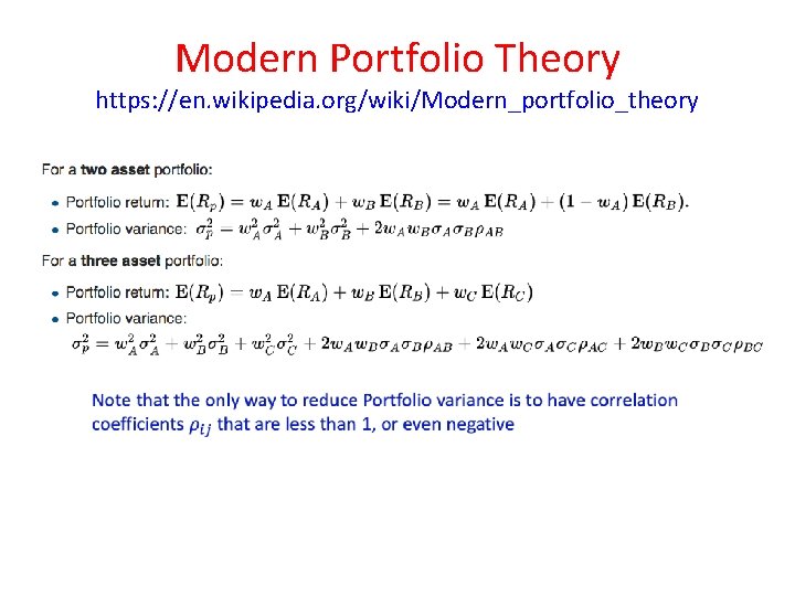
Modern Portfolio Theory https: //en. wikipedia. org/wiki/Modern_portfolio_theory

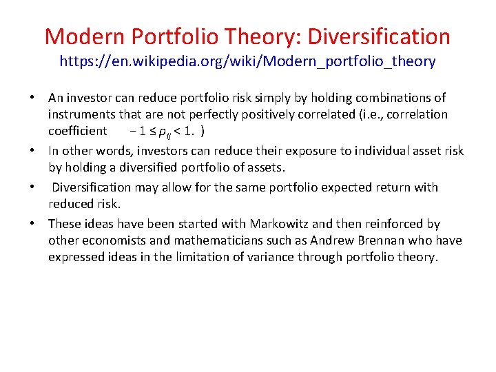
Modern Portfolio Theory: Diversification https: //en. wikipedia. org/wiki/Modern_portfolio_theory • An investor can reduce portfolio risk simply by holding combinations of instruments that are not perfectly positively correlated (i. e. , correlation coefficient − 1 ≤ ρij < 1. ) • In other words, investors can reduce their exposure to individual asset risk by holding a diversified portfolio of assets. • Diversification may allow for the same portfolio expected return with reduced risk. • These ideas have been started with Markowitz and then reinforced by other economists and mathematicians such as Andrew Brennan who have expressed ideas in the limitation of variance through portfolio theory.

Modern Portfolio Theory: Diversification https: //en. wikipedia. org/wiki/Modern_portfolio_theory • If all the asset pairs have correlations of 0, they are perfectly uncorrelated • Thus the portfolio's return variance is the sum over all assets of the square of the fraction held in the asset times the asset's return variance (and the portfolio standard deviation is the square root of this sum). • If all the asset pairs have correlations of 1, i. e. they are perfectly positively correlated, then the portfolio's volatility is the sum of each asset's volatility weighted by its fraction held in the portfolio. • This is the maximum volatility the portfolio of these assets would reach.

Expected Utility https: //en. wikipedia. org/wiki/Expected_utility_hypothesis • In economics, game theory, and decision theory the expected utility hypothesis, concerning people's preferences with regard to choices that have uncertain outcomes (gambles), states that if specific axioms are satisfied, the subjective value associated with an individual's gamble is the statistical expectation of that individual's valuations of the outcomes of that gamble. • Initiated by Daniel Bernoulli in 1738, this hypothesis has proved useful to explain some popular choices that seem to contradict the expected value criterion (which takes into account only the sizes of the payouts and the probabilities of occurrence), such as occur in the contexts of gambling and insurance. • Until the mid-twentieth century, the standard term for the expected utility was the moral expectation, contrasted with "mathematical expectation" for the expected value. • Each investor is assumed to have an individual utility function u(W) with respect to ownership of an asset W

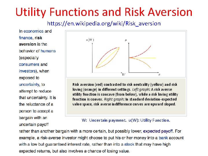
Utility Functions and Risk Aversion https: //en. wikipedia. org/wiki/Risk_aversion Risk aversion (red) contrasted to risk neutrality (yellow) and risk loving (orange) in different settings. Left graph: A risk averse utility function is concave (from below), while a risk loving utility function is convex. Right graph: In standard deviation-expected value space, risk averse indifference curves are upward sloped. W: Uncertain payment. u(W): Utility Function.

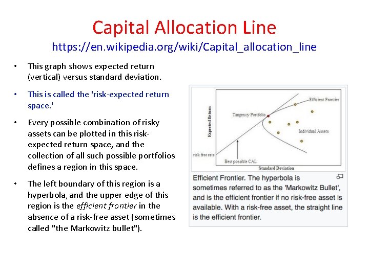
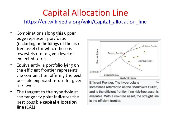
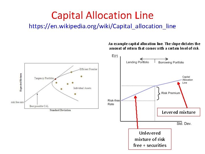
Capital Allocation Line https: //en. wikipedia. org/wiki/Capital_allocation_line • This graph shows expected return (vertical) versus standard deviation. • This is called the 'risk-expected return space. ' • Every possible combination of risky assets can be plotted in this riskexpected return space, and the collection of all such possible portfolios defines a region in this space. • The left boundary of this region is a hyperbola, and the upper edge of this region is the efficient frontier in the absence of a risk-free asset (sometimes called "the Markowitz bullet").

Capital Allocation Line https: //en. wikipedia. org/wiki/Capital_allocation_line • Combinations along this upper edge represent portfolios (including no holdings of the riskfree asset) for which there is lowest risk for a given level of expected return. • Equivalently, a portfolio lying on the efficient frontier represents the combination offering the best possible expected return for given risk level. • The tangent to the hyperbola at the tangency point indicates the best possible capital allocation line (CAL).

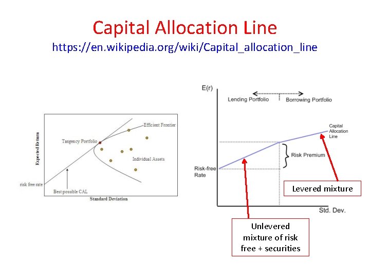
Capital Allocation Line https: //en. wikipedia. org/wiki/Capital_allocation_line Levered mixture Unlevered mixture of risk free + securities

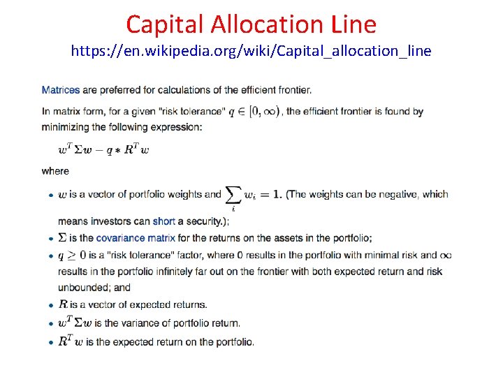
Capital Allocation Line https: //en. wikipedia. org/wiki/Capital_allocation_line

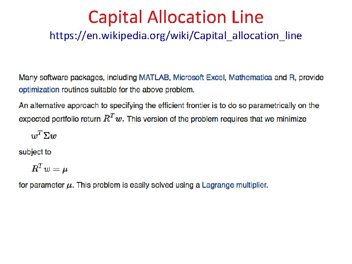
Capital Allocation Line https: //en. wikipedia. org/wiki/Capital_allocation_line

Risk Free Asset and Capital Allocation Line https: //en. wikipedia. org/wiki/Modern_portfolio_theory • The risk-free asset is the (hypothetical) asset that pays a risk-free rate. • In practice, short-term government securities (such as US treasury bills) are used as a risk-free asset, because they pay a fixed rate of interest and have exceptionally low default risk. • The risk-free asset has zero variance in returns (hence is risk-free) • It is also uncorrelated with any other asset (by definition, since its variance is zero). • As a result, when it is combined with any other asset or portfolio of assets, the change in return is linearly related to the change in risk as the proportions in the combination vary.

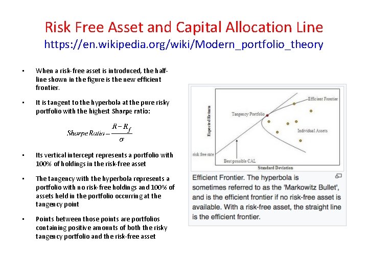
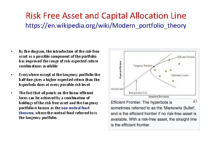
Risk Free Asset and Capital Allocation Line https: //en. wikipedia. org/wiki/Modern_portfolio_theory • When a risk-free asset is introduced, the halfline shown in the figure is the new efficient frontier. • It is tangent to the hyperbola at the pure risky portfolio with the highest Sharpe ratio: • Its vertical intercept represents a portfolio with 100% of holdings in the risk-free asset • The tangency with the hyperbola represents a portfolio with no risk-free holdings and 100% of assets held in the portfolio occurring at the tangency point • Points between those points are portfolios containing positive amounts of both the risky tangency portfolio and the risk-free asset

Capital Allocation Line https: //en. wikipedia. org/wiki/Capital_allocation_line An example capital allocation line. The slope dictates the amount of return that comes with a certain level of risk. Levered mixture Unlevered mixture of risk free + securities

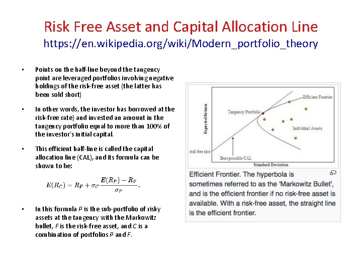
Risk Free Asset and Capital Allocation Line https: //en. wikipedia. org/wiki/Modern_portfolio_theory • Points on the half-line beyond the tangency point are leveraged portfolios involving negative holdings of the risk-free asset (the latter has been sold short) • In other words, the investor has borrowed at the risk-free rate) and invested an amount in the tangency portfolio equal to more than 100% of the investor's initial capital. • This efficient half-line is called the capital allocation line (CAL), and its formula can be shown to be: • In this formula P is the sub-portfolio of risky assets at the tangency with the Markowitz bullet, F is the risk-free asset, and C is a combination of portfolios P and F.

Risk Free Asset and Capital Allocation Line https: //en. wikipedia. org/wiki/Modern_portfolio_theory • By the diagram, the introduction of the risk-free asset as a possible component of the portfolio has improved the range of risk-expected return combinations available • Everywhere except at the tangency portfolio the half-line gives a higher expected return than the hyperbola does at every possible risk level. • The fact that all points on the linear efficient locus can be achieved by a combination of holdings of the risk-free asset and the tangency portfolio is known as the one mutual fund theorem, where the mutual fund referred to is the tangency portfolio.

“Two Mutual Fund” Theorem https: //en. wikipedia. org/wiki/Modern_portfolio_theory • One key result of the above analysis is the two mutual fund theorem. • This theorem states that any portfolio (risk-reward) on the efficient frontier can be generated by holding a combination of any two given portfolios on the frontier • The latter two given portfolios are the "mutual funds" in theorem's name. • So in the absence of a risk-free asset, an investor can achieve any desired efficient portfolio even if all that is accessible is a pair of efficient mutual funds.

“Two Mutual Fund” Theorem https: //en. wikipedia. org/wiki/Modern_portfolio_theory • If the location of the desired portfolio on the frontier is between the locations of the two mutual funds, both mutual funds will be held in positive quantities. • If the desired portfolio is outside the range spanned by the two mutual funds, then one of the mutual funds must be sold short (held in negative quantity) while the size of the investment in the other mutual fund must be greater than the amount available for investment • The excess would be funded by the borrowing from the other fund.